Visual DMS simulation

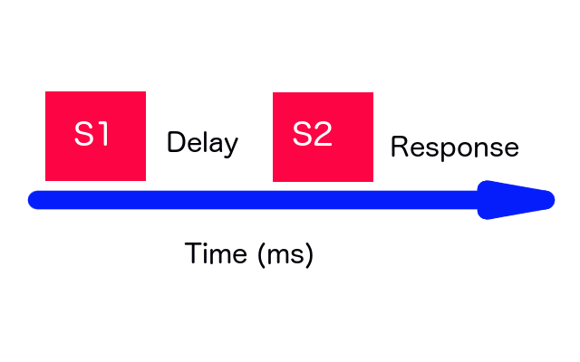
The following tutorial will show you how to install LSNM and perform a visual Delayed Match-to-Sample (DMS) simulation. As shown in the figure below, the DMS experiment to be simulated consists of a visual stimulus (S1) being presented to a subject, followed by a delay period during which time no stimulus is presented. At the end of the delay period, a second visual stimulus (S2) is presented to the subject, after which the subject must respond whether S1 and S2 are the same or different (Response).

Because the input module to our visual neural network (LGN) is composed of 81 units in the form of a 9x9 matrix, we need to organize our visual inputs in a 9x9 grid. We will initialize the units of our grid to zero and, in order to turn on selected units within the grid, we will assigning values of 0.92 to those units. For this tutorial, we will make use of inputs representing two-dimensional object shapes, all of them arranged in 9x9 grids and located in the script visual_model/script_to_replicate_Horwitz_2005_Fig_3.py (This script replicates Figure 3 of Horwitz et al, 2005).

In this tutorial, we will simulate one single trial.

NOTE: If you already have a working copy of LSNM, go directly to STEP 2

1. Download a copy of LSNM to your local workstation

• Launch Firefox or another web browser available on your local Unix workstation and copy/paste the following internet address (or just click on the highlighted link if you are in a browser already): https://github.com/NIDCD/lsnm_in_python.

• When the LSNM Github page displays, click on the button Download ZIP located on the right sidebar. Click on Save File to download the zip file containing the LSNM code to your Downloads folder.

• Inspect your downloads folder to make sure you have downloaded the LSNM files. There should be a file called lsnm-master.zip in it.

• Unzip the file in your preferred location:

    $ unzip lsnm-master.zip
  

• Change the name of the lsnm directory (to keep the sim executable from having problems with the special character -:

    $ mv lsnm-master lsnm
  

• NOTE: If you do not have access to an internet browser you can grab a copy of the LSNM repository by typing the following command on your local Unix workstation. Please note that at a directory called sim will be created in the directory where you are currently located:

    $ git clone https://github.com/NIDCD/lsnm_in_python.git
  

2. Move to a directory that contains simulated subject input data:

    $ cd lsnm_in_python/visual_model/subject_11

3. Make a directory called 'tutorial' and move to it

    $ mkdir tutorial
    $ cd tutorial

4. Now execute the simulator:

    $ python2.7 ../../../simulations/sim.py &

A GUI window will be displayed on the screen.

Please select your model as visual_model/model.txt in the "Model Description File" field, your weights as visual_model/subject_11/weightslist.txt in the "Weights List File" field, and your script as visual_model/script_to_replicate_Horwitz_2005_Fig_3.py in the "Simulation script File" field.

Leave the "File containing neural net" field empty. You would use this field (instead of using "Model Description File" and Weights List File") to specify a single file (of type JSON) that contains the description of a model and weights among regions.

Do not select "Use TVB Connectome" or "Vary weights to create new subject" at this point. The "Use TVB Connectome" option will embed the given LSNM nodes into a given connectome and run both LSNM and TVB simulators simultaneously. The "Vary weights to create a new subject" will multiply all weights by a given factor (usually a random number between 0.95 and 1.0) to create a new set of weights that will represent a "new" simulated subject.

Now, press the "Run" button.

5. Plot your output:

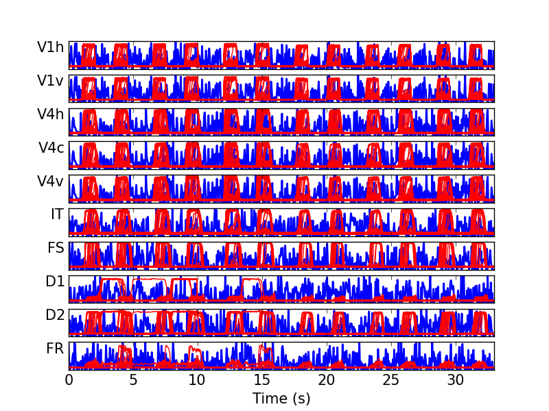
    $ python2.7 ../../../visualization/plot_neural_visual.py &

After which you should be able to see the following plot:

6. Convert neural output to integrated synaptic activity (ISA):

    $ python2.7 ../../analysis/compute_syn_visual.py &

7. Convert ISA to fMRI BOLD timeseries (1.5T):

    $ python2.7 ../../analysis/compute_BOLD_balloon_model.py &

8. Compute Percent Signal Change:

    $ python2.7 ../../analysis/compute_PSC.py &

9. Compute functional connectivity using BOLD time series:

    $ python2.7 ../../analysis/func_conn_across_subjs_visual.py &

10. Convert neural output to ISA using 998 ROIs (intrinsic "non-task-related" neural activity):

    $ python2.7 ../../analysis/compute_syn_visual_998_regions.py &

11. Convert intrinsic ISA to intrinsic fMRI BOLD timeseries in 998 ROIs (3T):

    $ python2.7 ../../analysis/compute_BOLD_balloon_3T_0.25Hz.py &

12. Generate intrinsic functional connectivity (FC) matrices of three conditions (passive fixation, passive viewing, and Delayed match-to-sample task) along with graph theoretical metrics; display and save results:

    $ python2.7 ../../analysis/compare_PF_PV_DMS.py