• introduction
• installation
• algorithm
  • AFC
  • FlowLF
  • FlowDBSCAN
  • ScaleFC
• data
• result

The source code, data and figures for the paper: ScaleFC: a scale-aware geographical flow clustering algorithm for heterogeneous origin-destination data

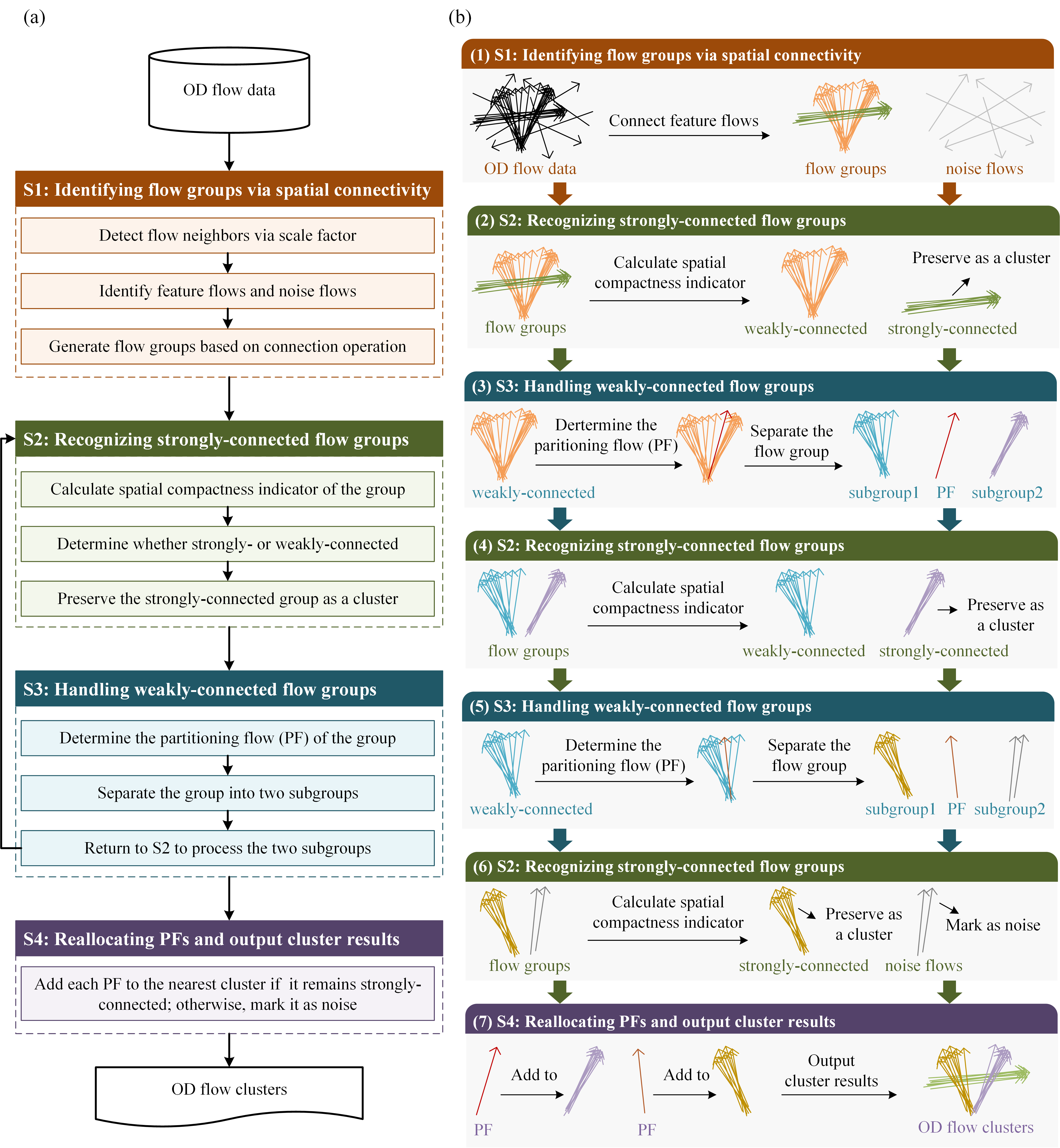
The workflow of ScaleFC:

introduction

• The directory algorithm includes four flow clustering algorithms used in this paper, i.e., AFC, FlowLF, FlowDBSCAN and ScaleFC.
• The directory data includes the six synthetic datasets and the real-word bike-sharing OD data used in this paper.
• The directory result includes the results of comparative experiment, parameter analysis and validation tests.
• Draw_flow.py is used to draw the flow clustering results.
• RunSyntheticData.py is used to run the synthetic data experiment.
• DrawFigures.ipynb records the code used to draw the figures in the paper.

installation

The codes only support python 3.9+, and use pip install -r requirements.txt to install essential packages. If you want to use jupyter, you can use pip install jupyter to install it.

algorithm

AFC

Agglomerative hierarchical flow clustering algorithm. A hierarchical flow clustering.

Input: 
   T = {Ti | 1 ≤ i ≤ n} – a set of origin-destination flows
   k – the number of nearest neighbors used in calculating distance.
Output: 
   A set of flow clusters C = {Cl | 1 < l << n}
Steps:
    1. Identify neighboring flows for each flow with a search radius k and create contiguous flow pairs, as explained in Section 3.2.
    2. Calculate the distance for each contiguity flow pair according to Equation 1, as explained in Section 3.3;
    3. Sort all contiguous flow pairs to an ascending order based on their distances;
    4. Initialize a set of flow clusters by making each flow a unique cluster, i.e. C = {Cl} and Cl = {Ti}, 1 ≤ l ≤ n; and
    5. For each contiguity flow pair (p, q), following the above ascending order:
        a. Find the two clusters Cx and Cy that p and q belong to: p ∈ Cx and q ∈ Cy;
        b. Calculate the distance dist(Cx, Cy) between Cx and Cy (see text below for detail); and
        c. If x ≠ y and dist(Cx, Cy) < 1, merge them: Cx = Cx∪Cy and C = C\Cy

Paper Reference: Zhu, Xi, and Diansheng Guo. “Mapping Large Spatial Flow Data with Hierarchical Clustering.” Transactions in GIS 18, no. 3 (June 2014): 421–35.

How to use:

from algorithm.AFC import flow_cluster_AFC
OD = ...
# to specify k manually
label = flow_cluster_AFC(OD, k=5) 
# to determin k by the condition that at least 95% flows have 1 neighbor and at least 70% of flows have 7 neighbors.
label = flow_cluster_AFC(OD, k=None, determin_k_by_m=True, at_least_m=(1, 7), at_least_ratio=(0.95, 0.7)) 

FlowLF

Use flow L-Function to cluster flows, a statistics-based flow clustering.

Main steps of the algorithm:

1. Determine the best radius using global L-function derivative
2. Calculate the local K-Function under the best radius
3. Identify core flows Monte Carlo test
4. Cluster the core flows by connected mechanism

Paper Reference: Shu H. et al. (2021). “L-function of geographical flows.” International Journal of Geographical Information Science 35(4), 689–716.

How to use:

from algorithm.FlowLF import flow_cluster_LF
OD = ...
# to specify the radius range and step size
labels = flow_cluster_LF(OD, radius_low=1, radius_high=5, radius_step=0.1, significance=0.05, MonteCarloTest_times=199)

FlowDBSCAN

FlowDBSCAN, implemented by scikit-learn. A density-based flow clustering.

Paper reference: Tao R. and Thill J.-C. (2016). “A Density-Based Spatial Flow Cluster Detection Method.” International Conference on GIScience Short Paper Proceedings 1.

How to use:

from algorithm.FlowDBSCAN import flow_cluster_dbscan
OD = ...
label = flow_cluster_dbscan(OD, eps=0.5, min_flows=5, n_jobs=-1)

ScaleFC

ScaleFC: a scale-aware geographical flow clustering algorithm for heterogeneous origin-destination data. A density-based flow clustering.

Steps:
    (1) Eliminate noise flows and identify flow groups via spatial connectivity measurement; 
    (2) Recognize the strongly-connected flow groups using the spatial compactness indicator. The strongly-connected flow groups are assigned as the final clusters, while the remain groups are treated as weakly-connected flow groups; 
    (3) Identify partitioning flows (PFs) within the generated weakly-connected flow groups to detect potential strongly-connected groups; 
    (4) Reallocate all partitioning flows to nearest flow clusters and output cluster results.

How to use:

from algorithm.ScaleFC import flow_cluster_ScaleFC
OD = ...
# to specify k manually
label = flow_cluster_ScaleFC(OD, scale_factor=0.1, min_flows=5)

data

Name	OD file	Label file
Dataset A	DataA.txt	DataA-label.txt
Dataset B	DataB.txt	DataB-label.txt
Dataset C	DataC.txt	DataC-label.txt
Dataset D	DataD.txt	DataD-label.txt
Dataset E	DataE.txt	DataE-label.txt
Dataset F	DataF.txt	DataF-label.txt

How to read datasets:

import numpy as np
OD_A = np.loadtxt('DataA.txt', delimiter=',')
real_label = np.loadtxt('DataA-label.txt', delimiter=',', dtype=int)

result

• adaption_results.csv is the result of the section adaption methods of scale factor and MinFlows.
• impact_of_two_parameters.csv is the result of ARI scores of the section impact of two parameters.
• ScaleFC_each_step_time.csv summarizes the time of each step of ScaleFC.
• ScaleFC-para-nonpara-time.csv stores the execuation time of ScaleFC with and without parallel computing.
• synthetic_clustering_resuls.csv is the result of four algorithms on synthetic datasets.
• time-complexity-500-5000-100-xxxx.csv stores the time complexity of four methods on datasets of varying size (small-scale).
• time-complexity-5500-20000-500-xxxx.csv stores the time complexity of four methods on datasets of varying size (large-scale).