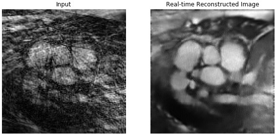
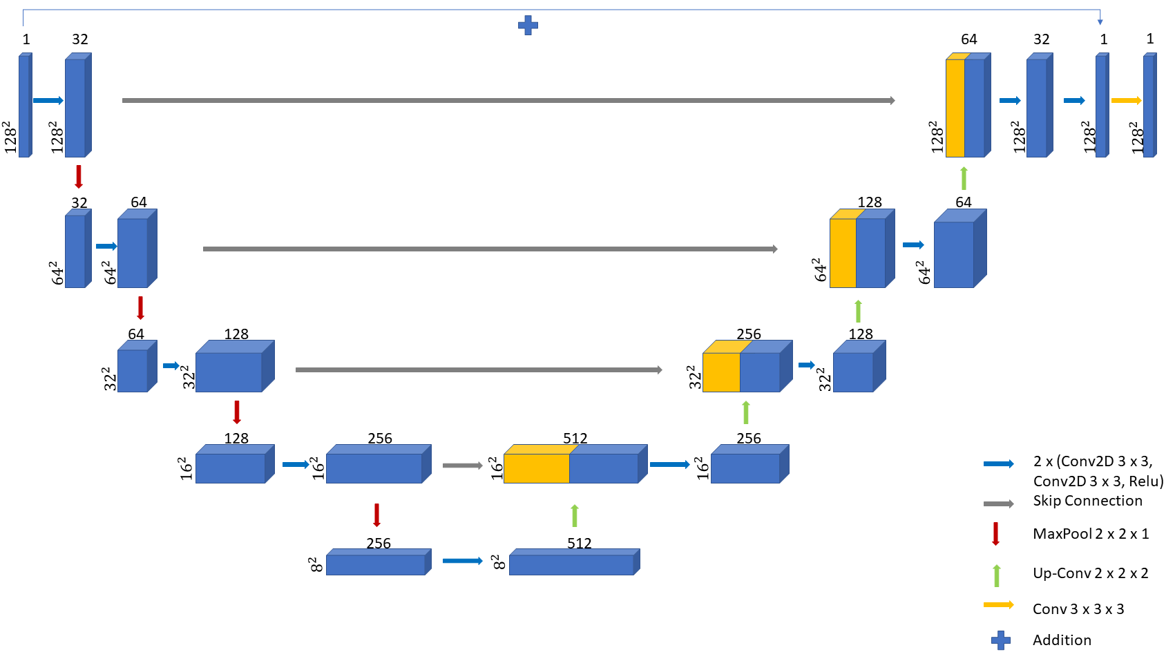
Classic Cardiovascular Magnetic Resonance takes a long time to obtain images over multiple heartbeats. Real-time CMR is faster than the classic one, but the data acquired is often of low spatial and temporal resolution. In this project, three UNets are used to produce MRI image reconstruction, namely, UNet3D, UNet2D1D, and UNet2D2D(below).
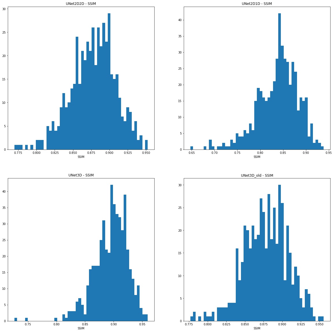
 The models were trained only on 66% of the original dataset, and I picked the top 3 settings by SSIM value in each network architecture. Comparison of different settings:
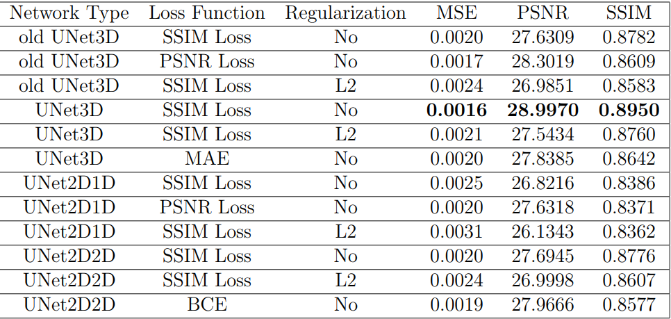
Note that the proposed UNet2D2D network architecture has only 1/3 parameters of UNet3D, and the SSIM loss is dominant among other loss functions.
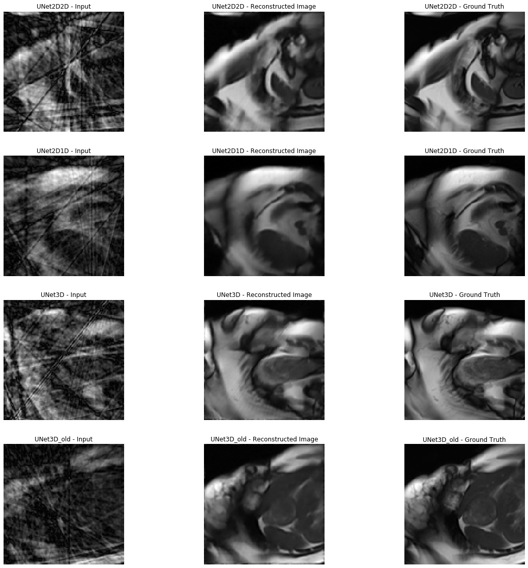
Best reconstructed images of each network architecture:
The configuration file training_config.yaml allows users to configure the training tasks and the hyperparameters in the network. Tensorboard logs and Tensorflow serving models are produced in the output folder by default.
Install CUDA Toolkit 10.0 as this is require for Tensorflow-gpu==1.14.0
Create an Anaconda environment, then in the activated environment, run
pip install -r requirements.txt
The above command should install all the dependencies required for training the model.
If you want to use docker to serve your model or use my pre-trained model. Please install Docker, Nvidia-Docker and Nvidia-container-runtime by following the installation instruction provided on your machine.
A script run_docker.sh is provided for you to run the Docker image on your machine.
Example Usage:
#!/bin/bash

MODEL_NAME='UNet2D2D'
SOURCE='/home/wentao/tensorflow_serving_model/models/'$MODEL_NAME
TARGET='/models/'$MODEL_NAME

docker run --runtime=nvidia -p 8501:8501 \
--mount type=bind,source=$SOURCE,target=$TARGET -e\
MODEL_NAME=$MODEL_NAME -t tensorflow/serving:latest-gpu &
In
'/home/wentao/tensorflow_serving_model/models/UNet2D1D'
Create a version number like 1, then copy and paste the content from the tf_serving folder into the created folder.
Then run the script:
sudo ./run_docker.sh
Open the example Jupyter Notebook docker_prediction.ipynb and have fun!
Example predictions:
A typical training task will look like below.
- task_name: 'UNet2D2D_MSE_loss_no_regularization'
  task_type: 'train_and_predict'
  email_notification: true
  input_data_path:
    x_train: './data/input_train.h5'
    y_train: './data/truth_train.h5'
    x_test: './data/input_test.h5'
    y_test: './data/truth_test.h5'
    x_val: './data/input_validation.h5'
    y_val: './data/truth_validation.h5'
    saved_network_weights:
  network_settings:
    network_type: 'UNet2D2D'
    batch_size: 1
    epochs: 20
    loss: 'MSE'
    metrics:
              - 'ssim'
    optimizer:
      type: 'Adam'
      learning_rate: 1.0e-04
    regularization:
      type: 'l2'
      parameters:
                 - 1.0e-05
    early_stopping:
      use: true
      patience: 2
      min_delta: 1.0e-02
output_data_dir: './keras_training'- task_name is used in notifications and constructing the output folder.
- task_type has three available options: 'train', which trains and store the model but not predicting the x_test. 'train_and_predict', which also produces a result.h5 file after prediction. 'predict', which only loads the model's weights and perform prediction.
- email_notification If this is set to True, you will receive email notifications at the beginning of the job and each task, when an exception is triggered, the end of each task and the job.
- input_data_path: These are for the input data paths.
- network_type: It specifies the model to use in the task, available options are UNet3D, UNet2D1D, UNet2D2D and UNet3D_old.
- batch_size: Network hyperparameters.
- epochs: Network hyperparameters.
- loss: It can be set to any losses by Keras in a string or my custom losses, 'psnr_loss' and 'ssim_loss'.
- metrics: It expects a list of strings, again, any metrics by Keras can be used, and my custom metrics, 'ssim' and 'psnr' are also available.
- optimiser: type: By now only two optimisers are implemented, 'Adam' and 'RMSprop'
- optimizer: learning_rate: Optimizer parameter.
- regularisation: type: Now, there are five options. 'l2', 'l1', 'l1_l2', 'batch_norm', and 'instance_norm', 'dropout' and 'dropblock'.
- regularisation: parameters: It expects a list of values, for example for 'dropblock', the parameters are keep_prob and block_size, so [0.8, 3] should be set in YAML format. Note that these layers are added after all convolutional layers by default.
- early_stopping: use: Set to true if you want to use the early stopping callback.
- early_stopping: patience: early_stopping parameter
- early_stopping: min_delta: early_stopping parameter
- output_data_dir: The directory where all the output data is stored.
It supports running the tasks consecutively so that you can add more than one tasks in the configuration file.
If you want to enable the email notification, please modify the file
./config/sample_email_config.yaml
Fill in the credentials and the receiver's email address.
smtp_server: 'smtp-mail.outlook.com'
smtp_server_port: 587
sender_email_address: ''
sender_email_password: ''
receiver_email_address: ''
then rename it to
email_config.yaml
It sends you emails when the task starts, ends and when it catches an exception.
You can either activate your virtual environment and run
conda activate python3.7
python train.py
alternatively, modify the bash script train.sh to activate your virtual environment then run the training so that you can type
sudo ./train.sh
You can also specify the GPUs you want to use in the bash script file. I have not added tf.distribute.MirroredStrategy due to I has only got one GPU now.
My machine has 16 GB RAM and RTX 2060 8GB graphics card, and most of the training can be run under such setup.
If you want to drop the SSH connection after you set up the job, run.
sudo ./nohup.sh
The output folder looks like this by default.
./keras_training/UNet2D2D_SSIM_loss_no_regularization/20190818-075223/
It has the following format:
output_data_dir/task_name/time/
If you run a 'train_and_predict' task by default, you will get
- tf_serving folder which contains the model that can be used by Tensorflow serving.
- predictions folder which includes a single h5 file named result.h5 which contains the prediction result.
- model_weights folder which contains the weights of the final trained model.
- logs folder which contains logs created by Tensorboard callback, which can be viewed by Tensorboard.
- checkpoints folder, which contains the weights of the model after each epoch.
- training_history pickle file, which contains the loss of the training in a python dictionary.
The evaluation result of my experiments is provided in a pickle file,## combined_evaluation_result.pkl , which contains an OrderedDict object.
In this OrderedDict, the result is stored in this format:
# task_name: [mse, nrmse, psnr, ssim, the_highest_ssim, the_lowest_ssim]
# The best result by ssim is in the first entry,
# the second-best by ssim is in the second entry etc.

# For example, the first two entries are:
OrderedDict([('UNet3D_SSIM_loss_no_regularization',
              [0.0015715675069023715,
               0.1598351978462956,
               28.996996515891965,
               0.8949767388036913,
               0.9595823120725895,
               0.7263687220098991]),
             ('UNet2D2D_SSIM_loss_no_regularization',
              [0.00199017724690729,
               0.17560795468353496,
               27.69450816257319,
               0.877606626530342,
               0.952268952715654,
               0.7698848257240287]))
If you want to find the best model from your training, I have also provided two Jupyter Notebook files to help you do that, calculate_metrics.ipynb and combine_metrics.ipynb.
The Tensorboard callback is set below.
tensorboard_callback = tf.keras.callbacks.TensorBoard(log_dir=tensorboard_logdir, histogram_freq=2,
                                                      write_graph=True, write_grads=True, write_images=True,
                                                      batch_size=batch_size)
For individual training, run the following command in
tensorboard --_logdir_=/path/to/the/log/dir
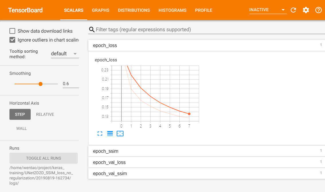
You can view the plot of the training loss and validation loss.
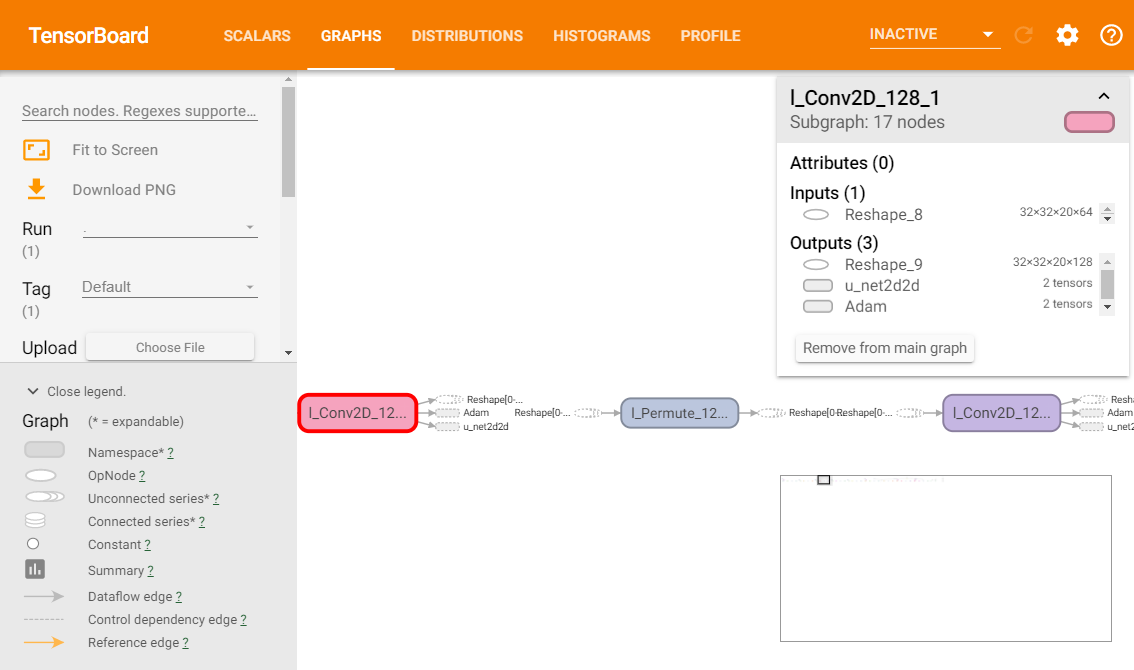
The firgure is showing a few nodes in the graph. You can understand how the layers are connected within the model if you check the whole graph in Tensorboard.
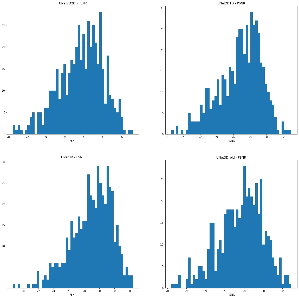
I provided a Jupyter Notebook network_result_visualiztion.ipynb to visualise the result. It plots the Input image, reconstrued image and the output image. It also plots histograms for mse, nrmse, psnr and ssim.
