-
Notifications
You must be signed in to change notification settings - Fork 16
Home
Extracting information from your fitted model can prove challenging, especially because of the dynamic internal structure of Bayesian-HMMs. This document is a work in progress to help outline some sensible approaches for extracting information from your model.
Let's assume you've fit a model that resembles the one from the README document:
import bayesian_hmm
import pandas as pd
import seaborn as sns
import matplotlib.pyplot as plt

# create emission sequences
base_sequence = list(range(5)) + list(range(5, 0, -1))
sequences = [base_sequence * 20 for _ in range(50)]

# initialise object with overestimate of true number of latent states
hmm = bayesian_hmm.HDPHMM(sequences, sticky=False)
hmm.initialise(k=20)

# use MCMC to estimate the posterior
results = hmm.mcmc(n=500, burn_in=100, ncores=3, save_every=10, verbose=True)Perhaps the most straightforward approach is to make use of the MAP-estimate. This simply involves finding the MCMC iteration that had the best likelihood, and extracting the model from this point in time. The benefit of this method is that the parameters themselves become fixed, allowing for straightforward inference on new data. The downside is that the full posterior distribution is lost, potentially losing some powerful information.
We can extract the MAP estimate very easily by looking through the likelihood in the results:
map_index = results['chain_loglikelihood'].index(min(results['chain_loglikelihood']))
state_count_map = results['state_count'][map_index]
hyperparameters_map = results['hyperparameters'][map_index]
parameters_map = results['parameters'][map_index]
The most important object ehre is the parameters_map dictionary. Using its p_initial, p_transition, and p_emission keys, we can extract the parameters that completely specify a (non-Bayesian) HMM. If we are using this approach, we may wish to remove the None state from each of these vectors, since the model no longer uses the hierarchical Dirichlet prior.
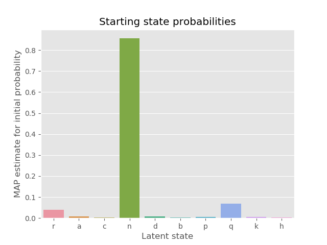
A common example of analysis may be in inspecting the starting state probabilities for the MAP-estimate:
p_initial_map = parameters_map['p_initial']
p_initial_map.pop(None)
p_initial = {k: v / sum(p_initial_map.values()) for k, v in p_initial_map.items()}
sns.barplot(x=list(p_initial.keys()), y=list(p_initial.values()))
plt.show()

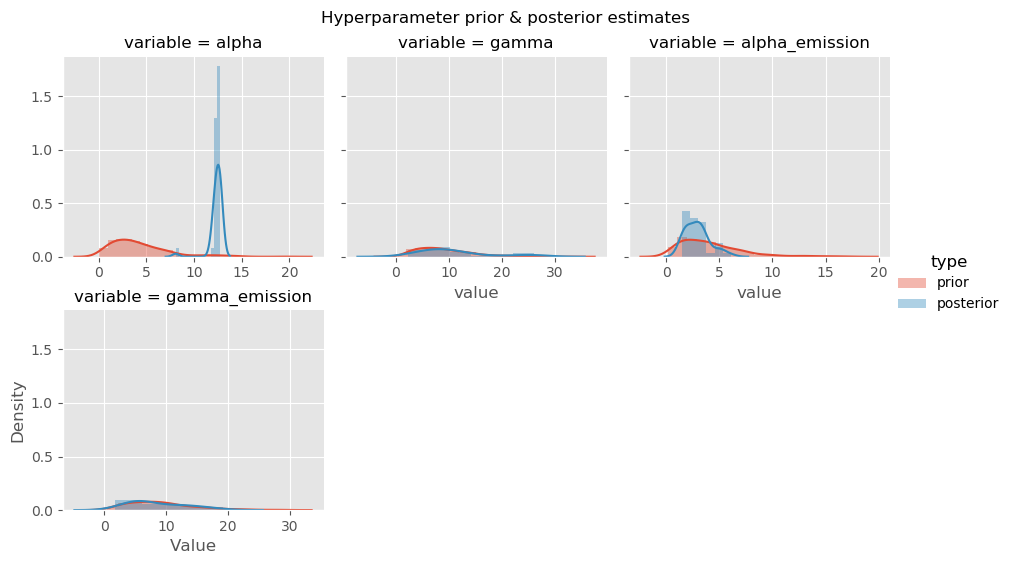
Another common step is to look at distributions of individual variables from the posterior distribution. This could be further advanced by producing pairwise densities or partial dependence plots.
hyperparam_posterior_df = (
    pd.DataFrame(results['hyperparameters'])
    .reset_index()
    .melt(id_vars=['index'])
    .rename(columns={'index': 'iteration'})
)
hyperparam_prior_df = pd.concat(
    pd.DataFrame(
        {'iteration': range(500), 'variable': k, 'value': [v() for _ in range(500)]}
    )
    for k, v in hmm.priors.items()
)
hyperparam_df = pd.concat(
    (hyperparam_prior_df, hyperparam_posterior_df),
    keys=['prior', 'posterior'],
    names=('type','index')
)
hyperparam_df.reset_index(inplace=True)

# advanced: plot sampled prior & sampled posterior together
g = sns.FacetGrid(
    hyperparam_df[hyperparam_df['variable'] != 'kappa'],
    col='variable',
    col_wrap=3,
    sharex=False,
    hue='type'
)
g.map(sns.distplot, 'value')
g.add_legend()
plt.show()
At any time, we can also inspect the parameters of the current system. These can be captured by accessing the attributes of the model object, but we can also print them conveniently using the HMM methods.
hmm.print_probabilities()╔═════╦═══════╗
║ S_i ║ Y_0 ║
╠═════╬═══════╣
║ r ║ 0.04 ║
║ a ║ 0.002 ║
║ c ║ 0.004 ║
║ n ║ 0.884 ║
║ d ║ 0.02 ║
║ b ║ 0.002 ║
║ p ║ 0.026 ║
║ q ║ 0.01 ║
║ k ║ 0.012 ║
║ h ║ 0.0 ║
╚═════╩═══════╝
╔Emission probabilities═════╦═══════╦═══════╦═══════╦═══════╗
║ S_i \ E_j ║ 0 ║ 1 ║ 2 ║ 3 ║ 4 ║ 5 ║
╠═══════════╬═══════╬═══════╬═══════╬═══════╬═══════╬═══════╣
║ r ║ 0.0 ║ 0.0 ║ 0.0 ║ 0.0 ║ 0.999 ║ 0.0 ║
║ a ║ 0.001 ║ 0.001 ║ 0.0 ║ 0.997 ║ 0.001 ║ 0.0 ║
║ c ║ 0.0 ║ 0.001 ║ 0.998 ║ 0.0 ║ 0.001 ║ 0.0 ║
║ n ║ 0.999 ║ 0.0 ║ 0.0 ║ 0.0 ║ 0.001 ║ 0.0 ║
║ d ║ 0.0 ║ 1.0 ║ 0.0 ║ 0.0 ║ 0.0 ║ 0.0 ║
║ b ║ 0.002 ║ 0.001 ║ 0.997 ║ 0.0 ║ 0.0 ║ 0.0 ║
║ p ║ 0.0 ║ 0.0 ║ 0.001 ║ 0.998 ║ 0.001 ║ 0.0 ║
║ q ║ 0.0 ║ 0.001 ║ 0.001 ║ 0.001 ║ 0.0 ║ 0.996 ║
║ k ║ 0.0 ║ 0.002 ║ 0.001 ║ 0.0 ║ 0.997 ║ 0.0 ║
║ h ║ 0.0 ║ 0.997 ║ 0.0 ║ 0.0 ║ 0.001 ║ 0.002 ║
╚═══════════╩═══════╩═══════╩═══════╩═══════╩═══════╩═══════╝
╔Transition probabilities═══╦═══════╦═══════╦═══════╦═══════╦═══════╦═══════╦═══════╦═══════╗
║ S_i \ E_j ║ r ║ a ║ c ║ n ║ d ║ b ║ p ║ q ║ k ║ h ║
╠═══════════╬═══════╬═══════╬═══════╬═══════╬═══════╬═══════╬═══════╬═══════╬═══════╬═══════╣
║ r ║ 0.001 ║ 0.002 ║ 0.0 ║ 0.001 ║ 0.0 ║ 0.002 ║ 0.001 ║ 0.988 ║ 0.004 ║ 0.0 ║
║ a ║ 0.993 ║ 0.0 ║ 0.0 ║ 0.002 ║ 0.001 ║ 0.0 ║ 0.0 ║ 0.001 ║ 0.001 ║ 0.0 ║
║ c ║ 0.0 ║ 0.991 ║ 0.001 ║ 0.002 ║ 0.001 ║ 0.001 ║ 0.0 ║ 0.0 ║ 0.002 ║ 0.001 ║
║ n ║ 0.002 ║ 0.001 ║ 0.001 ║ 0.0 ║ 0.993 ║ 0.0 ║ 0.0 ║ 0.0 ║ 0.001 ║ 0.0 ║
║ d ║ 0.0 ║ 0.001 ║ 0.997 ║ 0.0 ║ 0.0 ║ 0.0 ║ 0.001 ║ 0.0 ║ 0.0 ║ 0.0 ║
║ b ║ 0.0 ║ 0.003 ║ 0.0 ║ 0.002 ║ 0.0 ║ 0.002 ║ 0.003 ║ 0.0 ║ 0.0 ║ 0.99 ║
║ p ║ 0.001 ║ 0.001 ║ 0.0 ║ 0.0 ║ 0.0 ║ 0.997 ║ 0.0 ║ 0.0 ║ 0.001 ║ 0.0 ║
║ q ║ 0.0 ║ 0.001 ║ 0.0 ║ 0.001 ║ 0.001 ║ 0.0 ║ 0.001 ║ 0.001 ║ 0.992 ║ 0.002 ║
║ k ║ 0.0 ║ 0.001 ║ 0.0 ║ 0.001 ║ 0.0 ║ 0.001 ║ 0.991 ║ 0.003 ║ 0.002 ║ 0.001 ║
║ h ║ 0.001 ║ 0.001 ║ 0.002 ║ 0.992 ║ 0.0 ║ 0.0 ║ 0.001 ║ 0.001 ║ 0.0 ║ 0.001 ║
╚═══════════╩═══════╩═══════╩═══════╩═══════╩═══════╩═══════╩═══════╩═══════╩═══════╩═══════╝