1. Getting started
In this section, you will learn
- How to install Python using the Anaconda distribution.
- How to install GrainSizeTools.
- How to use Python through Jupyter Notebook or JupyterLab.
- How to interact with the script.
Note
The script does not require any previous knowledge of the Python programming language, but some knowledge of the basics is always an advantage. A general introduction to Python with a gentle learning curve can be found at the following web link: https://marcoalopez.github.io/Python_course/
GrainSizeTools requires the installation of Python 3, the Python scientific libraries NumPy SciPy, Pandas, Matplotlib, and JupyterLab. If you have no previous experience with Python, we recommend downloading and installing the Anaconda Python distribution, which is free and contains a comprehensive set of scientific Python libraries (> 5 GB disc space), including those needed to use GrainSizeTools. There are versions for Windows, MacOS and Linux.
https://docs.anaconda.com/free/anaconda/install/
Tip
If you have limited disk space or want more control over what you install, there is a distribution called Miniconda which installs only the Python packages you need. If you prefer to go to this route, click here for detailed instructions.
Once Anaconda is installed, launch the Anaconda Navigator and you will see that you have installed various scientifically oriented Integrated Development Systems (IDEs), including JupyterLab and the classic Jupyter Notebook. Clicking on any of these will open the corresponding application in your default web browser. The GrainSizeTools documentation is written assuming that you will be working using Jupyter Notebooks.
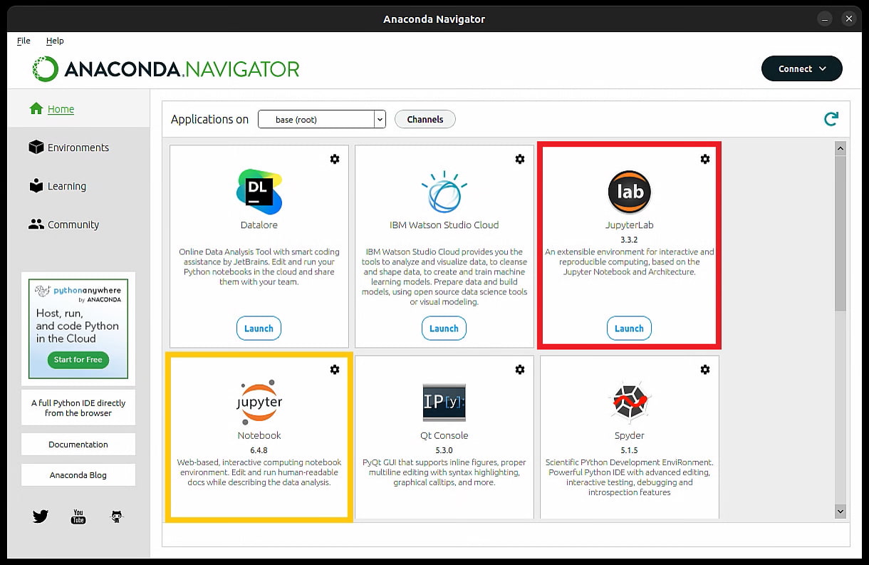
The appearance of the Anaconda navigator. Framed in red and orange are JupyterLab (preferred option) and Jupyter Notebooks (both should be installed by default in Anaconda). JupyterLab is the next generation of the Classic Jupyter Notebook user interface.
Tip
Using a dedicated application to work with Jupyter Notebooks
If you prefer to use a dedicated application instead of opening Jupyter Notebooks in your browser, there are several alternatives. Here we will mention two free alternatives:
- JupyterLab desktop: https://github.com/jupyterlab/jupyterlab-desktop/releases
This is a cross-platform desktop application for JupyterLab. It is the same application that opens in the browser but in an encapsulated application. You can find the user guide at the following link https://github.com/jupyterlab/jupyterlab-desktop/blob/master/user-guide.md. If you are a beginner, this is the easy road.
- Visual Studio Code (a.k.a. Vscode): https://code.visualstudio.com/
This is a free code editor that can be used with various programming languages including Python and supports Jupyter Notebooks via extensions. It has more advanced features than JupyterLab at the cost of being a bit more complicated to set up. More detailed instructions on how to use Jupyter Notebooks in Vscode at the following link https://code.visualstudio.com/docs/datascience/jupyter-notebooks
Note that both applications require Python to be installed on your operating system, i.e. it does not exempt you from the step of installing Python using Anaconda or any other distribution.
Once Python is installed, the next step is to download GrainSizeTools. Click on the download link below (there is also a direct link on the GrainSizeTools website).
https://github.com/marcoalopez/GrainSizeTools/releases
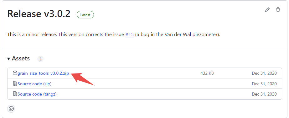
and download the latest version of the script by clicking on the zip file named grain_size_tools_v3.2.zip (numbers may change!) as shown below
Unzip the file and save the GrainSizeTools folder to a location of your choice. The GrainSizeTools folder contains various Python files (.py), a folder named DATA with a TXT file inside, and various Jupyter Notebooks (.ipynb files) that are templates for doing different types of grain size analysis.
Note
It is not necessary to download the zip files called Source code. They are for developers, not GrainSizeTools users.
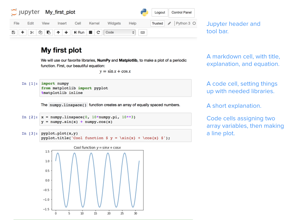
To improve reproducibility, we suggest working with the Jupyter Notebooks templates provided within the script, especially if you have no previous experience with the Python programming language. A Jupyter Notebook is a document that can contain executable code, equations (LaTeX), visualisations and narrative text so that the user bring together data, code, figures and prose in a single document. This is ideal for generating reports and including them as supplementary material in your publications so that any researcher can reproduce your results.
A Jupyter notebook, starting with a markdown cell containing a title and an explanation (including an equation rendered with LaTeX). Three code cells produce the final inline plot. Image source: Teaching and Learning with Jupyter
Note
A detailed explanation of how Jupyter Notebooks work is beyond the scope of this wiki page. The aim here is to teach the minimum necessary for a user to be able to use the Jupyter Notebook templates that come with the script. In any case, it is recommended that the user becomes familiar with the use of Jupyter Notebooks. There are excellent tutorials on the web explaining how to use Jupyter Notebooks, here are some suggestions:
-
JupyterLab official documentation: https://jupyterlab.readthedocs.io/en/latest/user/interface.html
-
https://www.youtube.com/watch?v=HW29067qVWk This is a video that explains in a clear, entertaining and concise way how to install and use a Jupyter Notebook, the usage part starts at about 4:20. For the tutorial, Corey uses the classic Jupyter Notebook application instead of JupyterLab, but it works similarly.
-
more suggestions to come...
When you first open JupyterLab, you should see something similar to this
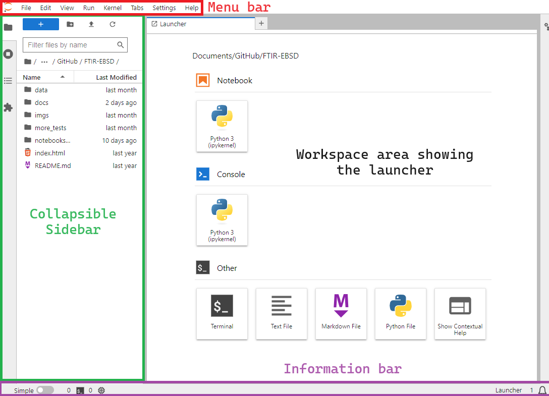
you should familiarise yourself with the following elements:
-
The Menu Bar at the top of the screen, highlighted in red, with familiar drop-down menus such as “File”, “Edit”, “View”, etc.
-
The Workspace Area currently displaying the Launcher. This allows users to access the Console, the Terminal or create new Notebooks, Python, Text, or Markdown files.
-
The Collapsible left Sidebar, highlighted in green, contains a File Browser, along with other items such as lists of running tabs and kernels, notebook table of contents, and the Extensions Manager.
-
The Information Bar highlighted in purple and located below.
At this point, use the launcher to create your first Jupyter Notebook.
When you create a notebook, you'll find an empty greyish cell at the top. These cells can be used for writing code, text (which is called markdown), or raw content. When you click in a cell, it turns white with a blinking cursor to indicate that it's ready for editing. The type of cell is shown in the top bar of the current tab. You can change the cell type at any time.
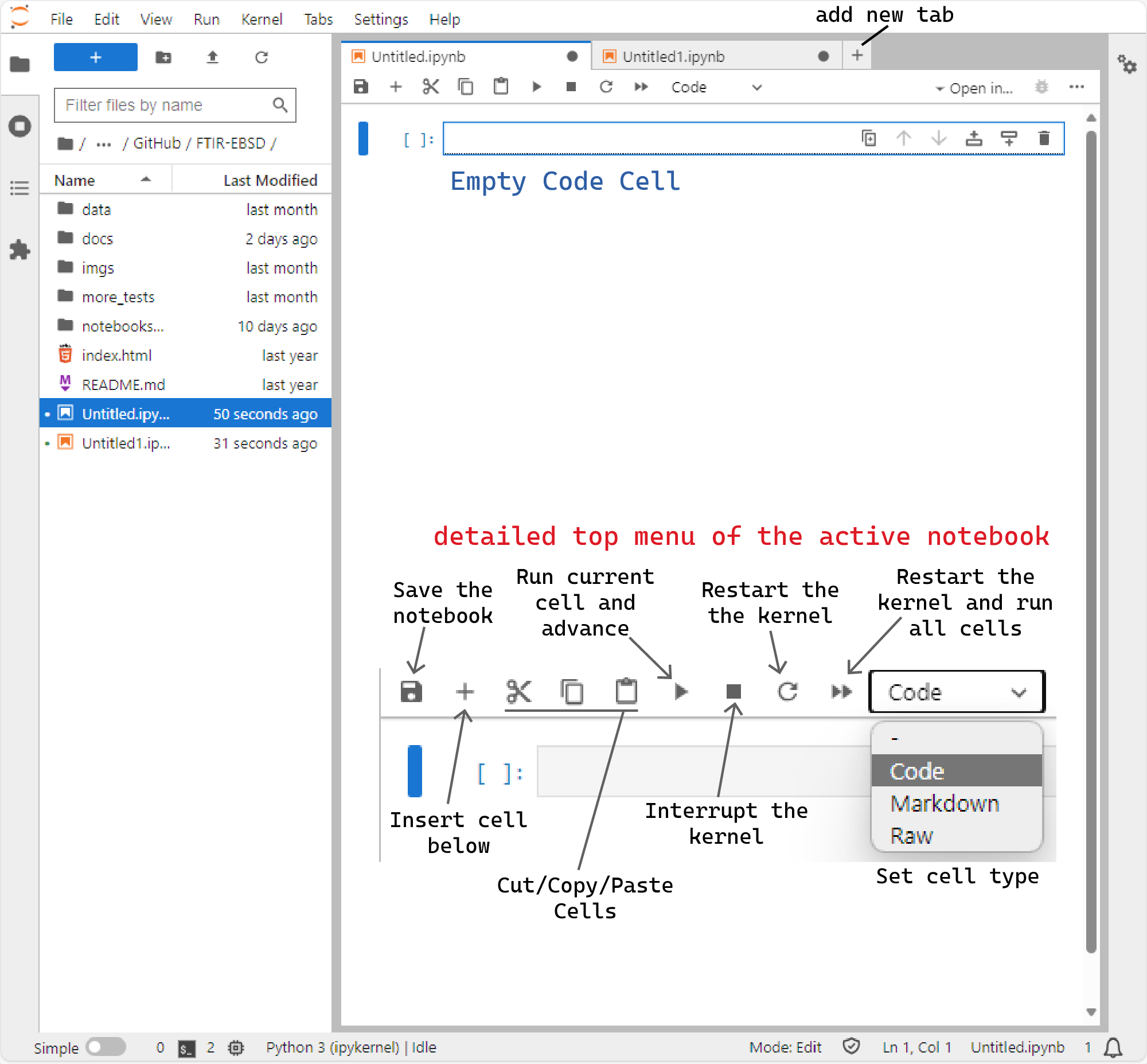
JupyterLab interface at a glance. More info at https://jupyterlab.readthedocs.io/en/latest/user/interface.html#the-jupyterlab-interface
If it's a code cell, you can write Python code in it. When you run the cell by pressing Shift+Enter the code gets executed, and any results appear just below the cell. The Shift+Enter action will also create a new empty cell just below it. If it is a markdown cell, you can use plain text with Markdown formatting to write your own annotations. When you're ready, press Shift+Enter and the text will be rendered and appear fully formatted. It will also create a new empty cell below it. Repeat this as many times as you need. Alternatively to the Shift+Enter command, one can run any selected cell clicking on the Play icon in the top bar of the notebook or using Ctrl/Cmd+Enter if you want to execute the cell and not added a new one below.
On the top right-hand side of any selected cell, you will see the following icons
![]()
These icons perform the following actions (in order from left to right): (i) create a duplicate of the current cell, (ii) move this cell up, (iii) move this cell down, (iv) insert an empty cell above, (v) insert an empty cell below, (vi) remove the cell.
When you open an edited notebook, for example the notebook templates that come with the script, you can edit any cell by clicking on the cell you want to modify and executing it once you have finished editing it.
Note
For any other questions about the JupyterLab interface, working with Jupyter files (creating, opening, renaming, etc.), we refer you to the official JupyterLab documentation here:
https://jupyterlab.readthedocs.io/en/latest/user/interface.html
Since version 3.2.0, the script consists of six Python files, three Jupyter notebook templates, a text-based YALM file (i.e. the piezometric database) and a folder named DATA, all contained in a folder named GrainSizeTools plus the version.
-
GrainSizeTools.py: This file imports all the modules needed for the script to fully describe grain size populations. -
averages.py: This module contains a set of functions for calculating different types of averages and confidence intervals. -
plot.py: This module contains a set of functions for generating various ad hoc plots used by the script. -
stereology.py: This module contains a set of functions to approximate true grain size distributions from sectional measurements using stereological methods. -
template.py: This file contains the default (Matplotlib) parameters used by the script to generate plots. -
piezometers.py: This file contains the methods to load the piezometric database and the methods to access and apply the various piezometric relationships. It is loaded independently of the other modules. Refer to the piezometry module documentation for more details.
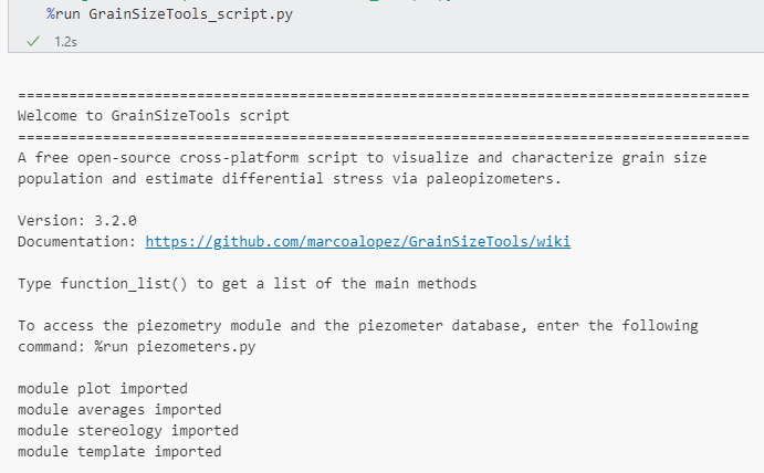
Once you run the GrainSizeTools.py in the Jupyter Notebook cell using the %run command, you will see information about all the imported modules, as well as some basic information as shown below:
As indicated in the information above, you can get a list of the different functions by using the following command:
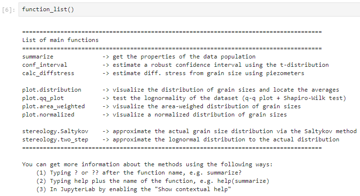
Note that to access some methods it is necessary to write the name of the module first, followed by a dot and then the name of the function or method to be used. (module.method()), for example:
plot.qqplot()In this case, this would read as follows: from the plot module use the qqplot function. Inside the parentheses would be the inputs required by the function. We will see the functionality of all the methods and look at these inputs in detail throughout the tutorial.
If you want to get detailed information about a method, use the single or double question mark an run the cell as follows:
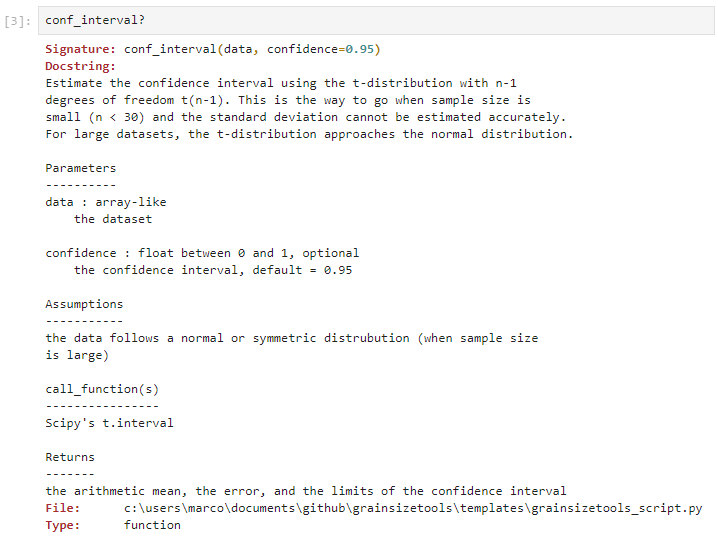
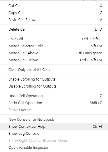
Alternatively, you can open the Contextual Help window to see all this information interactively (i.e. as soon as you type a method) in a separate window. To open it, right-click on the mouse and select "Show Contextual Help" (see example below) or press Ctrl+I.
In the GrainSizeTools folder, you'll find a subfolder called DATA. This is where you should store any grain size data you want to analyse. While it's not strictly necessary, it is a desirable for reproducibility. In addition, the templates for grain size analysis assume by default that all the data to be processed is located in this folder, although if wanted this can easily be changed.
Important
The GrainSizeTools script is not intended to deal with microscopic images but to quantify and visualize grain size populations and estimate stresses via paleopiezometers. It is, therefore, necessary to measure the grain diameters or the cross-sectional of the grains in advance and store them in a text (CSV, TXT, TSV) or excel file.
If the source of your data are images, we strongly recommend using the ImageJ application or one of its different flavours (see here). ImageJ-type applications are public domain image processing programs widely used in scientific research and run on all operating systems. This wiki includes a short tutorial on how to measure the areas of the grain profiles with ImageJ. The combined use of ImageJ and GrainSizeTools script is intended to ensure that all data processing steps are done through free and open-source programs/scripts that run under any operating system.
If you are dealing with EBSD data instead, we encourage you to use the MTEX toolbox for grain reconstruction and extracting the grain size data.
The GrainSizeTools folder contains three different notebook templates depending on the type of study you want to perform:
- quantification of grain size distributions (
grain_size_analysis_template.ipynb) - approximation of grain size distributions using stereological methods (
stereology_analysis_template.ipynb), - paleopiezometry (
paleopizometry_template.ipynb).
The notebooks contain practical examples on how to perform a grain size analysis. The user only has to change some parameters in the cells to adapt them to their study case and delete everything that is not needed. Once this is done, all the data structure and outputs will be contained in a single folder and the data handling procedures in a single fully reproducible document that can be exported to other formats (PDF, HTML, etc.) if necessary. When using this workflow, you should ideally copy the entire GrainSizeTool folder (<<1 MB), i.e. the code, the subfolder structure and the notebooks, for each grain size study you perform.
In a nutshell, once you have everything installed, open JupyterLab or Jupyter Notebooks and in the file manager go to the location where the script and templates are. Open the Jupyter template you want to use and follow the instructions in the template. That's it.
Caution
In the notebook, you can run cells in any order by selecting them and pressing Shift+Enter. But, when you share your notebook, it's best practice for reproducibility to run cells in the order they're shown. To do this, you can restart the kernel and then go to the menu bar and click on Run > Run All (the top menu of the notebook also has two icons for this purpose). This helps prevent unexpected issues if you're using variables between cells and improve reproducibility. Just be cautious when changing the order.
The file piezometric_database.yaml contains all the piezometric relationships. This database is easily modifiable as long as the YALM format is preserved. This can be done with any plain text editor. Refer to the piezometry module documentation for more details.
One of the most common tasks you'll do when interacting with the GrainSizeTools script is to load data into the Jupyter notebook. For this we will use the Pandas library, tool for reading and manipulating tabular datasets. Pandas will allow you to load structured data into an object called DataFrame, which is a two-dimensional labelled data structure, which will then allow you to interact with the GrainSizeTools script.
Here’s how you can import data from CSV and Excel files in a Jupyter notebook:
1. Importing Pandas (If needed):
First, you need to import the Pandas library. When you run the GrainSizeTools script the Pandas library is already imported as pd, so normally you don't need to do anything, otherwise you will need to import Pandas as follows
import pandas as pd2. Read a CSV/TSV/TXT file:
One common task is reading data from CSV (Comma Separated Values) or other text file types containing the data. Pandas read_csv() methods allows you to read a CSV file and convert it into a DataFrame. Here’s a basic example:
dataset_01 = pd.read_csv("filename.csv")In the example above, the method reads the file "filename.csv" from your current working directory, i.e. the directory where the notebook is located, and stores the data in a DataFrame named dataset_01. If the file is located elsewhere, you should replace this with the full or the relative path to the file. For example, if your file is in the DATA folder, as advised above, you should specify:
dataset_01 = pd.read_csv("DATA/filename.csv")Note that the DATA folder has been added to the path because it is in the current working directory. If the file were located elsewhere, you would need to specify the full path. The path can be either an absolute path or a path relative to your current working directory where the notebook resides (as in the example).
Tip
Once you loaded the data, call the DataFame or use the method head() , e.g. dataset_01.head(), to view the first few rows of your DataFrame to confirm successful import.
3. Using other delimiters:
A delimiter is a character that separates values in a text file. The most common delimiter is a comma, which is the one assumed by the read_csv() method. If your file uses a different delimiter, you can specify it using the delimiter or sep parameter. For example, if your fields are separated by tabs, you can read your file like this:
dataset_01 = pd.read_csv("DATA/file.tsv", delimiter="\t")In the example above, '\t' represents a tab character.
other common delimiters include:
- Tabs (
'\t') - Semicolons (
;) - Pipes (
|) - Spaces (` `)
Remember, it’s important to know what delimiter is used in your file to correctly read the data into a DataFrame. If you’re unsure, you can open the file in a text editor and check.
4. Column names:
By default, the read_csv function in Pandas assumes that the first row of your CSV/TSV file contains the column names for your DataFrame. This is controlled by the header parameter, which defaults to 0, indicating the first row. If your CSV doesn't have a header row with column names, read_csv will assign generic names like "Unnamed: 0", "Unnamed: 1", etc. to the columns. You can explicitly set header=None in read_csv to indicate there's no header row, and then provide your own column names using the names parameter:
dataset_01 = pd.read_csv("DATA/file.csv", header=None, names=["col1", "col2", "col3"])5. Skipping rows
Sometimes CSV files contains metadata or other non-data information at the beginning. In this case, the skiprows parameter allows you to specify the number of rows to skip from the beginning of the file. This can be useful if your CSV file contains metadata or other non-data information at the beginning. For example, if the first three rows of your CSV file are headers and comments, you can skip them as follows:
# Skipping the first three rows in the file
dataset_01 = pd.read_csv('file.csv', skiprows=3)
Note
For a deeper dive into read_csv options and functionalities, refer to the Pandas documentation: https://pandas.pydata.org/pandas-docs/stable/generated/pandas.read_csv.html
6. Importing other file types:
Pandas can read other tabular file formats including Excel files. For example, to read Excel files Pandas has the read_excel() function. Here's the basic syntax:
dataset_02 = pd.read_excel("DATA/data.xlsx")