This repository contains a purely python-based Bloch-McConnell (BMC) simulation tool that can be used to simulate the evolution of the magnetization in various (exchanging) magnetic environments ('pools') under arbitrary radio-frequency (RF) irradiation. The tool was developed to simulate Chemical Exchange Saturation Transfer (CEST) or related spectra, but can be used for many other MR simulations as well.
The BMCTool utilizes the pulseq open file format to define and store all events (RF pulses, gradients, delays, ADCs) that shall be simulated. The scanner settings and characteristic properties of the magnetic environments (relaxation times, pool size fractions, exchange rates) are defined and stored in config-files in the YAML file format.
Every simulation requires exactly one seq-file (containing all events) and at least one config-file.
The BMCTool can be installed from PyPi using
pip install bmctool
To make sure that the installation was successful, you can run an example simulation that is provided with both, the installation using pip and GitHub. To run an example simulation, simply execute the following code:
from bmctool.simulate import sim_example
sim_example()
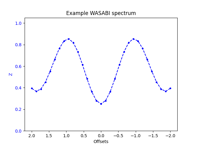
The sim_example function uses the WASABI.seq and config_wasabi.yaml example files. The generated plot should look like this:
All simulations using the BMCTool require a config file (in the yaml format) that includes all simulation settings and a sequence file (in the seq format), which defines the events to be simulated. An example seq-file and an example yaml file can be found in the library subfolder. For more information about config and sequence files and about the pulseq-cest-library, where both types of files are shared, please read the Pulseq-CEST Library section below.
If you created your own files or downloaded them from the pulseq-cest-library, you can start the simulation by running the following code:
from bmctool.simulate import simulate
config_path = '<path_to_your_config>'  # can be a str or a Path
seq_path = '<path_to_your_sequence>'  # can be a str or a Path
sim = simulate(config_file=config_path, seq_file=seq_path, show_plot=True)
The simulate function accepts several additional keyword arguments (**kwargs), that allow to adjust the plot. These are for example normalize (bool: toggle normalization), norm_threshold (value/list/array: threshold for normalization offsets), offsets (list/array: manually defined x-values), invert_ax (bool: toggle invert ax), plot_mtr_asym (bool:toggle plot MTR_asym) and title, x_label, y_label to control the lables.
The examples folder in the BMCTool GitHub repository contains some
further simulation examples as well as an example script to create your own WASABI.seq file. Please note that this
file will include an additional normalization offset at -300 ppm. To use this for normalization in the simulation,
simply add the kewword argument normalize=True to the simulate function.
The BMCTool was developed in parallel to the pulseq-cest project that aims to provide published and approved CEST saturation blocks in the pulseq open file format to enable an exact comparison of CEST saturation blocks with newly developed or adapted saturation blocks for reproducible research. The pulseq-cest project provides a MATLAB implementation and a python implementation. The python implementation uses the BMCTool and pypulseq for config and seq file handling. Both, the MATLAB and python implementation use the same Bloch-McConnell equation solver implemented in C++, which is much faster than the solver implemented in the BMCTool itself. For extensive simulations we thus recommend checking out the pulseq-cest implementations.
You will find several pre-defined and approved CEST pre-saturation schemes and simulation configs in the pulseq-cest-library GitHub repository. You can clone the library using
git clone https://github.com/kherz/pulseq-cest-library.git
or directly download the latest version as a ZIP file.
