Optical flow is the displacement map of pixels between two frames. It is a low-level analysis used in many computer vision programs.
Working with optical flow may be cumbersome:
- It is quite hard to represent it in a comprehensible manner.
- Multiple formats exist for storing it.
Flowpy provides tools to work with optical flow more easily in python.
We recommend using pip:
pip install flowpyThe main features of flowpy are:
- Reading and writing optical flows in two formats:
- Visualizing optical flows with matplotlib
- Backward and forward warp
This is the simplest example of how to use flowpy, it:
- Reads a file using flowpy.flow_read.
- Transforms the flow as an rgb image with flowpy.flow_to_rgb and shows it with matplotlib
import flowpy
import matplotlib.pyplot as plt

flow = flowpy.flow_read("tests/data/kitti_occ_000010_10.flo")

fig, ax = plt.subplots()
ax.imshow(flowpy.flow_to_rgb(flow))
plt.show()Sample image from the KITTI dataset
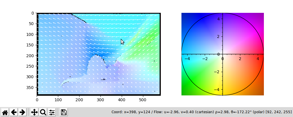
Flowpy comes with more than just RGB plots, the main features here are: - Arrows to quickly visualize the flow - The flow values below cursor showing in the tooltips - A calibration pattern side by side as a legend for your graph
flow = flowpy.flow_read("tests/data/Dimetrodon.flo")
height, width, _ = flow.shape

image_ratio = height / width
max_radius = flowpy.get_flow_max_radius(flow)

fig, (ax_1, ax_2) = plt.subplots(
    1, 2, gridspec_kw={"width_ratios": [1, image_ratio]}
)

ax_1.imshow(flowpy.flow_to_rgb(flow))
flowpy.attach_arrows(ax_1, flow)
flowpy.attach_coord(ax_1, flow)

flowpy.attach_calibration_pattern(ax_2, flow_max_radius=max_radius)

plt.show()Sample image from the Middlebury dataset
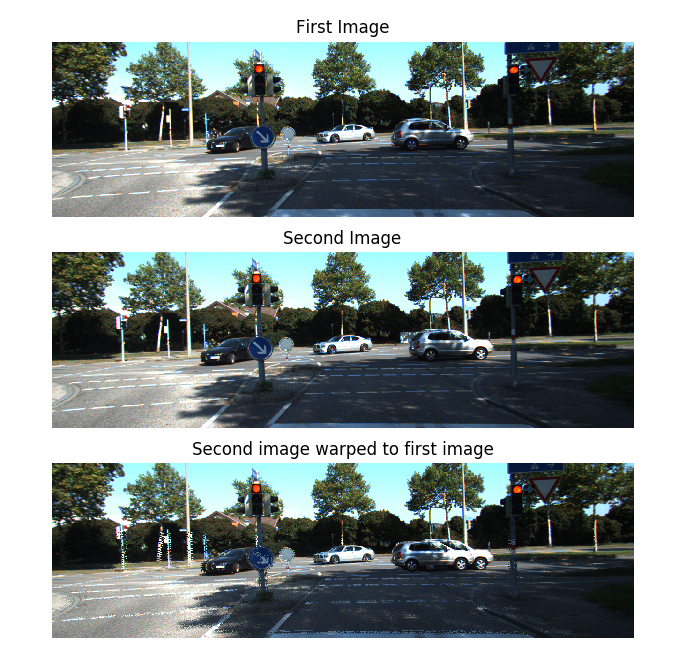
If you know the flow (first_image -> second_image), you can backward warp the second_image back to first_image.
flow = flowpy.flow_read("static/kitti_occ_000010_10.png")
first_image = np.asarray(Image.open("static/kitti_000010_10.png"))
second_image = np.asarray(Image.open("static/kitti_000010_11.png"))

flow[np.isnan(flow)] = 0
warped_first_image = flowpy.backward_warp(second_image, flow)

fig, axes = plt.subplots(3, 1)
for ax, image, title in zip(axes, (first_image, second_image, warped_first_image),
                            ("First Image", "Second Image", "Second image warped to first image")):
    ax.imshow(image)
    ax.set_title(title)
    ax.set_axis_off()

plt.show()Note that the artifacts in the warp are normal, they are caused by unknown flows and occlusions.
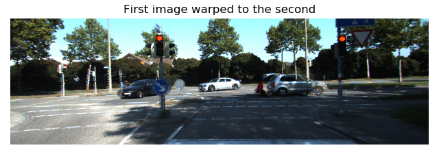
Forward warp is often less used as it is quite more complex. It relies on a k-nearest neighbor search instead of direct bi-linear interpolation.
forward_warp is about 10x slower than backward_warp but you still may find it useful.
flow = flowpy.flow_read("static/kitti_occ_000010_10.png")
first_image = np.asarray(Image.open("static/kitti_000010_10.png"))
second_image = np.asarray(Image.open("static/kitti_000010_11.png"))

flow[np.isnan(flow)] = 0
warped_second_image = flowpy.forward_warp(first_image, flow)

fig, ax = plt.subplots()

ax.imshow(warped_second_image)
ax.set_title( "First image warped to the second")
ax.set_axis_off()

plt.show()You can find the above examples in the examples folder. You can also look in tests.
If you encounter a bug or have an idea for a new feature, feel free to open an issue.
Most of the visualization and io handling has been translated from matlab and c code from the Middlebury flow code. Credits to thank Simon Baker, Daniel Scharste, J. P. Lewis, Stefan Roth, Michael J. Black and Richard Szeliski.


