Building Capacity and Generating Evidence for Climate Change Impacts on Soil, Sediments and Water Resources in Mountainous Regions
This tutorial consists of blocks of code for step-by-step building a calibrated Volumetric Water Content also know as soil moisture by combining Nuclear related Technique and Earth Observation Data. In this report the Cosmic-Ray Neutron Sensor (CRNS) and the C-Band Radar Sentinel 1 data over Peru and Bolivia will be used to calibrate a large scale spatio-temporal Soil Moisture. We will use Google Earth Engine (GEE) which is a free, cloud-based analysis of satellite data analysis with a catalogue of satellite imagery and geospatial datasets. All satellite data used in this study were processed in this cloud computing platform. A JavaScript application program interface (API) was used to analyze satellite data. However, Python and R versions can also be used.
The Cosmic Ray Neutron Sensor (CRNS) is an advanced Nuclear method that can estimate area-wide soil moisture, approximately 20ha by detecting and counting the number of slow neutrons in the soil and in the air just above the soil. These neutrons are produced by incoming high-energy cosmic rays from outside the solar system. This helps fill the need for spatial soil moisture information left by common point-based sensors. The CRNS in this study was installed at around 4,500 meters altitude, close to the eternal snow of the 6,088 meters high Huayna Potosi mountain in the C. ordillera Real.
Sentinel-1 (S1) Ground Range Detected (GRD) is the first of the five missions that the European Space Agency (ESA) developed for the Copernicus ini tiative (Fig.1) The S1 mission includes two C-band SAR imaging polar-orbiting satellites, providing continuous radar mapping of the globe regardless of the weather. The S1 mission provides data collection of a dual-polarization instrument. This collection includes: GRD calibrated ortho-corrected scenes, and each scene has one of 3 resolutions (10, 25 or 40 meters)4 band combinations (VV+VH and HH+HV) (corresponding to scene polarisation) 3 instrument modes. The C-band SAR has 5 days temporal resolution and covers the entire world’s land masses for land monitoring, emergency response, climate change and security. found that the Vertical-Vertical (VV) polarisation of Sentinel-1 is suitable for soil moisture monitoring, mainly because the VV polarisation is more sensitive to the soil contribution.
Sentinel-2 (S2) is a high-resolution, wide-swath imaging mission that supports Copernicus Land Monitoring research, such as vegetation, soil and water cover monitoring, as well as observation of inland waterways and coastal areas (Fig.1). Sentinel-2 imageries are acquired through two twin satellites (Sentinel-2A and Sentinel-2B), launched separately into synchronous polar orbit at an altitude of 786 km and evolving at 180° from each other. Each satellite is equipped with a Multi-Spectral Imager sensor (MSI) covering 13 spectral bands (from 443 nm to 2190 nm) with a field of view of 290 km, and a spatial resolution of 10 m (4 bands in the visible and near infrared domains), 20 m (6 bands in the near and short wavelength infra-red domain, NIR and SWIR), and 60 m (3 atmospheric correction bands). They monitor the variability of the Earth's surface conditions, or changes in vegetation with the seasons, in a high return time (10 days at the equator with one satellite and 5 days with the constellation of the two satellites). In this study, the Normalized Difference Vegetation Index (NDVI) was estimated . This vegetation index will allow users to follow vegetation biomass.
The first step is to either load the shapefiles of the study area or manually enter the coordinates of the CRNS installation site. Figure 1 shows the loading steps of the shapefiles of the area in Bolivia. The following code shows the predefined steps on top for visualization.
/***********************************************************************************************************
 * region of interest ROI based on the shapefile
 * definition of the coord of the point in Long and Lat
 * definition of the buffer zone of 14km around the ROI
***********************************************************************************************************/
var roi=ee.FeatureCollection('users/chaponda/Mexico/Contours-20m')
var lines=ee.FeatureCollection('users/chaponda/Mexico/Reach-Tuni-Condoriri-HuaynaPotosi')
var bolivia_point=ee.Geometry.Point([-68.28579402514282, -16.26308678038219])
var bolivia_buffer=bolivia_point.buffer(14000)
Map.setOptions('TERRAIN')
Map.centerObject(bolivia_point,11)
Map.addLayer(bolivia_buffer,{},'Foot Print')
Map.addLayer(roi,{},'Countours',true)
Map.addLayer(lines.draw('blue',1,1),{},'waterLine',true)
Fig. 2: representation of the study area where the Cosmic-ray neutron sensor is in Bolivia.
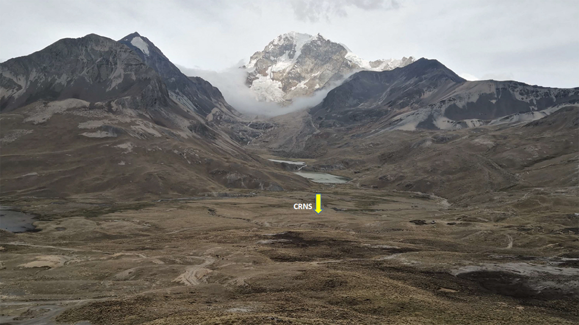
Fig.3: Photographic View of the site, from : https://www.iaea.org/newscenter/news/iaea-supports-study-of-bolivian-wetland-water-reserves-as-glaciers-melt
The boxcar filtering method was used to reduce signal noise and increase the spatial resolution of the model. In the code, the number 3 refers to the number of pixels ee. kernel.circle (3). A series of filtering (temporal filtering, spatial filtering, polarization filtering and ascending mode) was applied for data reduction. Then, a function is applied to crop all the images in interest and the print function displays the number of images available. It is important to just keep the ASCENDING mode of the SAR data and the VV polarization because soil moisture is more sensitive to the VV polarization than the VH polarization . in this example, the time interval between the current date and 4 years back was considered. the print function gives details information concerning the c-band satellite data as shown below in figure .4
var now=ee.Date(Date.now())
 var boxcar = ee.Kernel.circle(3);
 var soilmoisture = ee.ImageCollection("COPERNICUS/S1_GRD")
                   .filterBounds(bolivia_buffer)
                   .filter(ee.Filter.listContains('transmitterReceiverPolarisation', 'VV'))
                   .filter(ee.Filter.listContains('transmitterReceiverPolarisation', 'VH'))
                   .filter(ee.Filter.eq('orbitProperties_pass', 'ASCENDING'))
                   .filterDate(now.advance(-4,'years'),now)
                   .map(function(image){
                     return image.clip(bolivia_buffer)
                                 .select(['VV'])
                                 .convolve(boxcar)
                                 .multiply(0.0222)
                                 .add(0.4945)
                                 .rename('SSM')
                                 .copyProperties(image,['system:time_start'])
                   })

 print('collection information', soilmoisture)
Fig.4: Visualization of the metainformation or properties of the Sentinel-1 data
the following code allows visualizing the map of mean soil moisture in Bolivia. the visual parameters are set to minimum and maximum based on the 4 years annuals mean minimum and mean maximum value.
var visParam = {min:0.01,max: 1,palette:["red", "orange","green","blue"]}
Map.addLayer(ssm, visParam , 'Soil Moisture',true)
Map.addLayer(soilmoisture,visParam , 'Ssm T',true)
Fig. 5: Mapping spatial variation of soil moisture
The last step in this code is to extract the time series of VV polarization at the location of the CRNS (see fig.6). Time series of the VV component for five (5) years were extracted and data were exported to R for processing.
var chartSSM = ui.Chart.image.doySeriesByYear(soilmoisture,'SSM', bolivia_point.buffer(300), ee.Reducer.mean(), 10)
                .setChartType('ScatterChart')
                .setOptions({ title: 'Top Surface Soil Moisture ',
                vAxis: {title: 'VWC (cm3/cm3)'},hAxis: {title: 'Date'},
                legend: {position: 'left'}, })


print(chartSSM)
Fig.6: Example of 4 years(2021 to 2018) evolution of the soil moisture
This application allows the visualization of the Spatio-temporal series of soil moisture. Two buttons allow the user to point directly to the CRNS installation areas, namely Peru and Bolivia. These two buttons are located on the left side of the application. The user can click on a radius of 14 Km to visualize the temporal dynamics of the estimated soil moisture. For short periods of time over a year, it is possible to use the panel on the left, where one must choose a time interval (date 1, date 2) and click on the button on the far right to see the spatialization of soil moisture and the time series of two zones, one at high altitude and one at low altitude.
Fig. 7: illustration of all output of the Web GIS platform
https://sites.google.com/view/crnswetlandsandes
- Gorelick, N., Hancher, M., Dixon, M., Ilyushchenko, S., Thau, D., & Moore, R. Google Earth Engine: Planetary-scale geospatial analysis for everyone. Remote sensing of Environment, (2017). 202, 18-27.*
- Singh, A.; Gaurav, K.; Meena, G.K.; Kumar, S. Estimation of Soil Moisture Applying Modified Dubois Model to Sentinel-1; A Regional Study from Central India. Remote Sens. (2020), 12, 2266
- Drusch, M., Del Bello, U., Carlier, S., Colin, O., Fernandez, V., Gascon, F., ... & Meygret, A. Sentinel-2: ESA's optical high-resolution mission for GMES operational services. Remote sensing of Environment. (2012), 120, 25-36.
- Bauer-Marschallinger, B., Freeman, V., Cao, S., Paulik, C., Schaufler, S., Stachl, T., Modanesi, S., Massari, C., Ciabatta, L., Brocca, L., & Wagner, W. (2019). Toward Global Soil Moisture Monitoring With Sentinel-1: Harnessing Assets and Overcoming Obstacles. IEEE Transactions on Geoscience and Remote Sensing, 57(1), 520–539. https://doi.org/10.1109/TGRS.2018.2858004
- Chung, J., Lee, Y., Kim, J., Jung, C., & Kim, S. (2022). Soil Moisture Content Estimation Based on Sentinel-1 SAR Imagery Using an Artificial Neural Network and Hydrological Components. Remote Sensing, 14(3), 465. https://doi.org/10.3390/rs14030465
- Dari, J., Brocca, L., Quintana-Seguí, P., Casadei, S., Escorihuela, M. J., Stefan, V., & Morbidelli, R. (2022). Double-scale analysis on the detectability of irrigation signals from remote sensing soil moisture over an area with complex topography in central Italy. Advances in Water Resources, 161, 104130. https://doi.org/10.1016/j.advwatres.2022.104130
- Vather, T., Everson, C., & Franz, T. E. (2019). Calibration and Validation of the Cosmic Ray Neutron Rover for Soil Water Mapping within Two South African Land Classes. Hydrology, 6(3), 65. https://doi.org/10.3390/hydrology6030065
- Wieder, W., Shoop, S., Barna, L., Franz, T., & Finkenbiner, C. (2018). Comparison of soil strength measurements of agricultural soils in Nebraska. Journal of Terramechanics, 77, 31–48. https://doi.org/10.1016/j.jterra.2018.02.003