Face mask detection with Tensorflow CNNs

COVID-19 has been an inspiration for many software and data engineers during the last months. This project demonstrates how a Convolutional Neural Network (CNN) can detect if a person in a picture is wearing a face mask or not. As you can easily understand the applications of this method may be very helpful for the prevention and the control of COVID-19 as it could be used in public places like airports, shopping malls etc.

Defining the problem

Detecting if an image contains a person wearing a mask or not is a simple classification problem. We have to classify the images between 2 discrete classes: The ones that contain a face mask and the ones that do not.

The dataset

Hopefully, I found a dataset containing faces with and without masks online. It is available on this github link. It contains 1,376 images. 690 images show people with face masks and 686 images show people without face masks.

Image classification and CNNs

A bit of theoretical background first. Convolutional Neural Networks (CNN) are neural networks most commonly used to analyze images. A CNN receives an image as an input in the form of a 3D matrix. The first two dimensions corresponds to the width and height of the image in pixels while the third one corresponds to the RGB values of each pixel.

CNNs consist of the following sequential modules (each one may contain more than one layer)

1. Convolution
2. ReLu activation function
3. Pooling
4. Fully connected layers
5. Output layer

Convolution

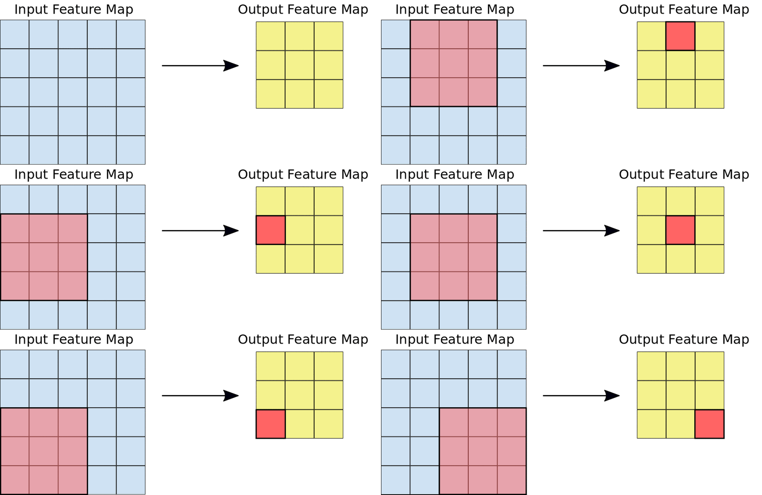
Convolution operation is an element wise matrix multiplication operation. Convolutional layers take the three-dimensional input matrix we mentioned before and they pass a filter (also known as convolutional kernel) over the image, applying it to a small window of pixels at a time (i.e 3x3 pixels) and moving this window until the entire image has been scanned. The convolutional operation calculates the dot product of the pixel values in the current filter window along with the weights defined in the filter. The output of this operation is the final convoluted image.

The following animation (found in Google developers portal) shows how the sliding o the window is performed over an image

The core of image classification CNNs is that as the model trains what it really does is that it learns the values for the filter matrices that enable it to extract important features (shapes, textures, colored areas etc) in the image. Each convolutional layer applies one new filter to the convoluted image of the previous layer that can extract one more feature. So, as we stack more filters, the more features the CNN can extract from an image.

ReLu activation function

After each convolution operation, CNN applies to the output a Rectified Linear Unit (ReLu) function to the convolved image. As you may remember from the Machine Learning 101 course in university, ReLu is very commonly used in machine learning applications because it introduces nonlinearity into the model. This helps our model to generalize better and avoid overfitting.

Pooling

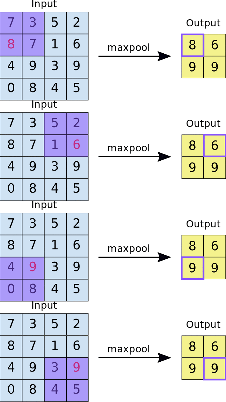
Pooling is the process where the CNN downsamples the convolved image by reducing the number of dimensions of the feature map. It does so to reduce processing time and the computing power needed. During this process, it preserves the most important feature information. There are several methods that can be used for pooling. The most common ones are Max pooling and Average pooling. In our application, we will use max pooling as it is the most effective most of the times. Max pooling is very similar to the convolution process. A windows slides over the feature map and extracts tiles of a specified size. For each tile, max pooling picks the maximum value and adds it to a new feature map.

The following animation (found in Google developers portal) shows how max pooling operation is performed.

Fully connected layers

After pooling, there is always one or more fully connected layers. These layers perform the classification based on the features extracted from the image by the previously mentioned convolution processes. The last fully connected layer is the output layer which applies a softmax function to the output of the previous fully connected layer and returns a probability for each class.

The general form of an image classification CNN is the one shown below:

Face mask detection

I used Tensorflow and Keras to create the CNN that classifies the images as with or without mask.

First, we need to randomly split the dataset in separate train / test sets. We do so with the following function:

def train_test_split(source, trainPath, testPath, split_size):
	dataset = []
	for crnImage in os.listdir(source):
		data = source + '/' + crnImage
		if(os.path.getsize(data) > 0):
			dataset.append(crnImage)
	train_len = int(len(dataset) * split_size)
	test_len = int(len(dataset) - train_len)
	shuffled = random.sample(dataset, len(dataset))
	train = dataset[0:train_len]
	test = dataset[train_len:len(dataset)]
	print("train images with mask:",len(train))
	print("test images without mask:",len(test))

  #copying train and test images in seaparate directories
	for trainDataPoint in train: 
		crnTrainDataPath = source + '/' + trainDataPoint
		newTrainDataPath =  trainPath + '/' + trainDataPoint
		copyfile(crnTrainDataPath, newTrainDataPath)

	for testDataPoint in test:
		crnTestDataPath = source + '/' + testDataPoint
		newTestDataPath =  testPath + '/' + testDataPoint
		copyfile(crnTestDataPath, newTestDataPath)

We then call it twice (one for the images that contain a mask and one fot the images that do not) with a train / test split of 80% (80% used for training and 20% for test).

train_test_split('data/with_mask', 'data/train/training_with_mask', 'data/test/test_with_mask',0.8)
train_test_split('data/without_mask','data/train/training_without_mask', 'data/test/test_without_mask',0.8)

The model

The definition of the model is presented below:

model = tf.keras.models.Sequential([
    Conv2D(32, 3, activation='relu', input_shape=(IMG_WIDTH, IMG_HEIGHT, 3)),
    MaxPooling2D(2,2),
    Conv2D(64, 3, activation='relu'),
    MaxPooling2D(2,2),
    Conv2D(128, 3, padding='same', activation='relu'),
    MaxPooling2D(2,2),
    Flatten(),
    Dropout(0.3), 
    Dense(256, activation='relu'),
    Dense(2, activation='softmax') # dense layer has a shape of 2 as we have only 2 classes 
])
model.compile(optimizer='adam', loss='binary_crossentropy', metrics=['accuracy'])

The model consists of 10 layers in total. The first 6 layers form 3 sequential Convolution - ReLu - Pooling groups. Then, a flatten layer is applied to reshape the output of the CNN to a single dimension. After the flatten layer, a dropout layer is applied. This layer randomly drops 30% (rate = 0.3) of the tensors in order to avoid overfitting. In the end, a fully connected (dense) layer is applied that classifies the images based on the features extracted in the previous layers of the CNN and the final layer outputs the probability of each class label.

We also use binary_crossentropy as the loss function because our data contain only 2 classes.

Training the model

We train the model with the following function. First, we open 2 training streams ("flows") from the 2 directories of train and test (validation) images. We also save checkpoints during training in separate directories for each checkpoint. Finally, we call the fit_generator function of the model and training begins. During the process we keep track of training and validation accuracy and loss (we will use the values later to plot learning curves).

def trainModel():
  training_dir = "data/train"
  train_datagen = ImageDataGenerator(rescale=1.0/255,
                                     rotation_range=40,
                                     width_shift_range=0.2,
                                     height_shift_range=0.2,
                                     shear_range=0.2,
                                     zoom_range=0.2,
                                     horizontal_flip=True,
                                     fill_mode='nearest')

  train_generator = train_datagen.flow_from_directory(training_dir, 
                                                      batch_size=10, 
                                                      target_size=(IMG_WIDTH, IMG_HEIGHT))
  validation_dir = "data/test"
  validation_datagen = ImageDataGenerator(rescale=1.0/255)
  validation_generator = validation_datagen.flow_from_directory(validation_dir, 
                                                           batch_size=10, 
                                                           target_size=(IMG_WIDTH, IMG_HEIGHT))
  checkpoint = ModelCheckpoint('model-{epoch:03d}.model',monitor='val_loss',verbose=0,save_best_only=True,mode='auto')

  history = model.fit_generator(train_generator,
                                epochs=epochs,
                                validation_data=validation_generator,
                                callbacks=[checkpoint])
  global acc
  acc = history.history['accuracy']
  global val_acc
  val_acc = history.history['val_accuracy']
  global loss
  loss = history.history['loss']
  global val_loss
  val_loss = history.history['val_loss']

Then, we label the outputs of the CNN ans apply colors to the results (red for without mask, green with mask) as follows:

labels_dict = {0:'without mask',1:'with mask'}
color_dict = {0:(0,0,255),1:(0,255,0)}

Implementing face detection

Inspired by this face and mask detection article, I used the OpenCV framework to implement live face detection using the default webcam of the computer. I used the very common Haar Feature-based Cascade Classifiers for detecting the features of the face. This cascade classifier is designed by OpenCV to detect the frontal face by training thousands of images.

Face and mask detection is performed in the following code (courtesy of Gurucharan M K).

# Initializing webcam to live preview face mask detection ROIs on faces
# Seen this in this repo https://github.com/mk-gurucharan/Face-Mask-Detection
face_clsfr = cv2.CascadeClassifier('haarcascade_frontalface_default.xml')

labels_dict = {0:'without mask',1:'with mask'}
color_dict = {0:(0,0,255),1:(0,255,0)}

size = 4
webcam = cv2.VideoCapture(0)
classifier = cv2.CascadeClassifier('haarcascade_frontalface_default.xml')

while True:
    (rval, im) = webcam.read()
    im = cv2.flip(im,1,1) #Flip to act as a mirror

    # Resize the image to speed up detection
    mini = cv2.resize(im, (im.shape[1] // size, im.shape[0] // size))
    faces = classifier.detectMultiScale(mini)

    # Draw rectangles around each face
    for (x, y, w, h) in faces:
        face_img = im[y:(y+h)*size, x:(x+w) * size]
        resized=cv2.resize(face_img,(IMG_WIDTH, IMG_HEIGHT))
        normalized = resized / 255.0
        reshaped = np.reshape(normalized,(1,IMG_WIDTH,IMG_HEIGHT,3))
        reshaped = np.vstack([reshaped])
        result = model.predict(reshaped)
        
        label = np.argmax(result,axis=1)[0]
      
        cv2.rectangle(im,(x* size,y* size),((x+w)* size,(y+h)* size),color_dict[label],2)
        cv2.rectangle(im,(x * size,(y* size)-40),((x+w)* size,y* size),color_dict[label],-1)
        cv2.putText(im, labels_dict[label], (x* size + 10, (y* size)-10),cv2.FONT_HERSHEY_DUPLEX,0.8,(255,255,255),2)
        
    cv2.imshow('Mask Detection', im)
    key = cv2.waitKey(10)
    if key == 27:
        break
webcam.release()
cv2.destroyAllWindows()

Benchmarks

The learning curves (training and validation accuracy and loss) of the model are the following for 30 epochs of training: As you can see we achieved an accuracy of more than 98% in the validation dataset which is nice!

In my 2.5 GHz i7, 16 GB Ram MacBook Pro, the model took almost 17 minutes to train.

References

1. COVID-19: Face Mask Detection using TensorFlow and OpenCV
2. Mask images dataset
3. Google developer - ML Practicum: Image Classification
4. saama - Different Kinds of Convolutional Filters