Breast cancer is one of the most common types of cancer in the UK. According to NHS, about 1 in 8 women are diagnosed with breast cancer during their lifetime, and early detection will significantly increase the chance of recovery.
Goal: train machine learning models to predicts whether the cancer is benign or malignant based on a digital scan of the tumour cells.
The dataset used in this story is publicly available and was created by Dr. William H. Wolberg, physician at the University Of Wisconsin Hospital at Madison, Wisconsin, USA. To create the dataset Dr. Wolberg used fluid samples, taken from patients with solid breast masses and an easy-to-use graphical computer program called Xcyt, which is capable of perform the analysis of cytological features based on a digital scan. The program uses a curve-fitting algorithm, to compute ten features from each one of the cells in the sample, than it calculates the mean value, extreme value and standard error of each feature for the image, returning a 30 real-valuated vector.
The mean, standard error and “worst” or largest (mean of the three largest values) of these features were computed for each image, resulting in 30 features. For instance, field 3 is Mean Radius, field 13 is Radius SE, field 23 is Worst Radius.
Data exploration and feature engineering: involved data cleaning, i.e. handling of null values, checking class distribution and exploring collinearity in the dataset.
The final dataset included 9 variables: concave points_worst, radius_se, texture_worst, smoothness_worst, symetry_worst, concave points_se, symetry_mean, franctal_dimension_worst, compactness_se and diagnosis.
Due to the nature of the problem requiring to build a model which can classify the nature of the tumour as benign or malignant, we concluded that the most suitable ML algorithm is a classification one.
Considering that each record in the data was already labelled with the diagnosis, malignant(M) vs benign (B), we decided to experiment with supervised ML algorithms. Classification models used: logistic regression, decision tree, random forest, svm and Adaboost.
The data was split into training data (80% of the entire data set) and test data (20% of the entire data set).
Confusion Matrix
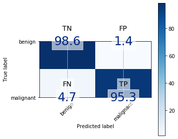
A confusion matrix is a summary of prediction results on a classification problem. The number of correct and incorrect predictions are summarized with count values and broken down by each class. A confusion matrix helps us gain an insight into how correct our predictions were and how they hold up against the actual values. The four values are true positive (predicted yes and actually was yes), true negative (predict no and actually was no), false positive (predicted yes and actually was no) and false negative (predicted no and actually was yes).
Confusion matrix for logistic regression:
Accuracy, precision, recall and F-1 score metrics were used to assess the performance of the models applied to the pre-processed breast cancer image data.
Accuracy and precision are two important factors to consider when taking data measurements. Both accuracy and precision reflect how close a measurement is to an actual value, but accuracy reflects how close a measurement is to a known or accepted value, while precision reflects how reproducible measurements are, even if they are far from the accepted value.
- Accuracy is the ratio of the total number of correct predictions and the total number of predictions.
- Precision is the ratio between the True Positives and all the Positives. For our problem statement, that would be the measure of patients that we correctly identify having breast cancer out of all the patients actually having it.
- Recall is the measure of our model correctly identifying True Positives. Thus, for all the patients who actually have breast cancer, recall tells us how many we correctly identified as having a cancer.
- F1-score is the Harmonic mean of the Precision and Recall.
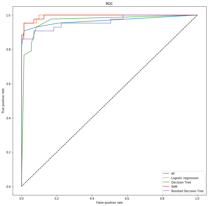
The ROC curve is a graphical plot that illustrates the diagnostic ability of a binary classifier system as its discrimination threshold is varied.
We plotted the ROC curce to assess the performce of the models as seen below. Area under the curve (AUC) represents degree or measure of separability. It tells how much model is capable of distinguishing between classes. Higher the AUC, better the model is at predicting 0s as 0s and 1s as 1s. By analogy, Higher the AUC, better the model is at distinguishing between patients with disease and no disease.
Highest recall, precision and F1-score: Logistic regression
Best AUC: SVM 0.87, this means that the model will be able to distinguish the patients with breast cancer and those without 87% of the time.
| Model | Precision | Recall | F-score |
|---|---|---|---|
| Logistic regression | 0.973719 | 0.973684 | 0.973621 |
| Decision Tree | 0.903367 | 0.903509 | 0.902763 |
| Random Forest | 0.956905 | 0.956140 | 0.955801 |
| SVM | 0.956905 | 0.956140 | 0.955801 |
| Boosted Decision Tree | 0.912281 | 0.912281 | 0.912281 |
Logistic regression model applied to a dataset of 8 characteristics derived from a tumour image aid to reconfirm malignant diagnosis, adding evidence to doctors' diagnosis of cancer.
├── LICENSE
├── Makefile           <- Makefile with commands like `make data` or `make train`
├── README.md          <- The top-level README for developers using this project.
├── data
│   ├── external       <- Data from third party sources.
│   ├── interim        <- Intermediate data that has been transformed.
│   ├── processed      <- The final, canonical data sets for modeling.
│   └── raw            <- The original, immutable data dump.
│
├── docs               <- A default Sphinx project; see sphinx-doc.org for details
│
├── models             <- Trained and serialized models, model predictions, or model summaries
│
├── notebooks          <- Jupyter notebooks. Naming convention is a number (for ordering),
│                         the creator's initials, and a short `-` delimited description, e.g.
│                         `1.0-jqp-initial-data-exploration`.
│
├── references         <- Data dictionaries, manuals, and all other explanatory materials.
│
├── reports            <- Generated analysis as HTML, PDF, LaTeX, etc.
│   └── figures        <- Generated graphics and figures to be used in reporting
│
├── requirements.txt   <- The requirements file for reproducing the analysis environment, e.g.
│                         generated with `pip freeze > requirements.txt`
│
├── setup.py           <- makes project pip installable (pip install -e .) so src can be imported
├── src                <- Source code for use in this project.
│   ├── __init__.py    <- Makes src a Python module
│   │
│   ├── data           <- Scripts to download or generate data
│   │   └── make_dataset.py
│   │
│   ├── features       <- Scripts to turn raw data into features for modeling
│   │   └── build_features.py
│   │
│   ├── models         <- Scripts to train models and then use trained models to make
│   │   │                 predictions
│   │   ├── predict_model.py
│   │   └── train_model.py
│   │
│   └── visualization  <- Scripts to create exploratory and results oriented visualizations
│       └── visualize.py
│
└── tox.ini            <- tox file with settings for running tox; see tox.readthedocs.io
Project based on the cookiecutter data science project template. #cookiecutterdatascience

