instability

library(tree)

library(parallel)

With the current model/set of parameters, things here are nowhere near as bad as they used to be. However, there is still some useful information here.

Try to establish what the equilubrium seed rain is.

p <- ebt_base_parameters()

p$add_strategy(new(Strategy))

p$seed_rain <- 1.1                       # Starting rain.

run <- function(seed_rain_in, p, schedule) {
  p$seed_rain <- seed_rain_in
  run_ebt(p, schedule)$seed_rains
}

run_collect <- function(seed_rain_in, p, schedule) {
  p$seed_rain <- seed_rain_in
  run_ebt_collect(p, schedule)
}

run_new_schedule <- function(w, p, schedule=NULL) {
  p$seed_rain <- w
  res <- build_schedule(p, schedule)
  unname(attr(res, "seed_rain")[,"out"])
}

1: Approach to equilibrium:

res <- equilibrium_seed_rain(p)

## 1: Splitting {34} times (141)
## 2: Splitting {12} times (175)
## *** 1: {1.1} -> {70.94} (delta = {69.84})
## 1: Splitting {44} times (141)
## 2: Splitting {34} times (185)
## 3: Splitting {24} times (219)
## 4: Splitting {14} times (243)
## 5: Splitting {3} times (257)
## *** 2: {70.94} -> {59.62} (delta = {-11.31})
## 1: Splitting {42} times (141)
## 2: Splitting {33} times (183)
## 3: Splitting {26} times (216)
## 4: Splitting {15} times (242)
## 5: Splitting {2} times (257)
## *** 3: {59.62} -> {59.89} (delta = {0.2692})
## *** 4: {59.89} -> {59.89} (delta = {-0.005533})
## *** 5: {59.89} -> {59.89} (delta = {3.182e-05})
## *** 6: {59.89} -> {59.89} (delta = {-7.99e-07})
## Reached target accuracy (delta 7.98969e-07 < 1.00000e-05 eps)

seed_rain_eq_in <- unname(res[["seed_rain"]][,"in"])

seed_rain_eq_out <- unname(res[["seed_rain"]][,"out"])

schedule1 <- res[["schedule"]]$copy()

approach <- t(sapply(attr(res, "progress"), "[[", "seed_rain"))

Sanity and time check

system.time(cmp <- run(seed_rain_eq_in, p, schedule1)) # ~10s

##    user  system elapsed 
##   5.680   0.023   5.801

cmp - seed_rain_eq_out # should be exactly zero

## [1] 0

Check that running the ebt with collection does not change things:

system.time(res_cmp <- run_collect(seed_rain_eq_in, p, schedule1)) # ~13s

##    user  system elapsed 
##   7.088   0.036   7.251

res_cmp$seed_rain - seed_rain_eq_out

## [1] 0

Then, in the vinicity of the root we should look at what the curve actually looks like, without adaptive refinement.

dr <- 1 # range of input to vary (plus and minus this many seeds)

seed_rain_in  <- seq(seed_rain_eq_in - dr,
                     seed_rain_eq_in + dr, length=31)

seed_rain_out <- unlist(mclapply(seed_rain_in, run, p, schedule1))

fit <- lm(seed_rain_out ~ seed_rain_in)

p2 <- p$copy() # modify fast control

p2$set_control_parameters(list(environment_light_tol=1e-6))

system.time(cmp2 <- run(seed_rain_eq_in, p2, schedule1)) # ~20s

##    user  system elapsed 
##  19.286   0.062  19.764

seed_rain_out2 <- unlist(mclapply(seed_rain_in, run, p2, schedule1))

fit2 <- lm(seed_rain_out2 ~ seed_rain_in)

p3 <- p$copy() # modify fast control

p3$set_control_parameters(list(ode_tol_rel=1e-5, ode_tol_abs=1e-5))

system.time(cmp3 <- run(seed_rain_eq_in, p3, schedule1)) # ~21s

##    user  system elapsed 
##  15.957   0.053  16.933

seed_rain_out3 <- unlist(mclapply(seed_rain_in, run, p3, schedule1))

fit3 <- lm(seed_rain_out3 ~ seed_rain_in)

p4 <- p$copy() # modify fast control

p4$set_control_parameters(list(plant_assimilation_rule=61))

system.time(cmp4 <- run(seed_rain_eq_in, p4, schedule1)) # ~13s

##    user  system elapsed 
##   10.49    0.03   10.59

seed_rain_out4 <- unlist(mclapply(seed_rain_in, run, p4, schedule1))

fit4 <- lm(seed_rain_out4 ~ seed_rain_in)

p5 <- p2$copy() # modify high-precision light environment

p5$set_control_parameters(list(plant_assimilation_rule=61))

system.time(cmp5 <- run(seed_rain_eq_in, p5, schedule1)) # ~24s

##    user  system elapsed 
##  24.701   0.051  25.059

seed_rain_out5 <- unlist(mclapply(seed_rain_in, run, p5, schedule1))

fit5 <- lm(seed_rain_out5 ~ seed_rain_in)

# fast, better light environment, better ode, better assimilation,

# better assimilation and better light environment

cols <- c("black", "red", "blue", "green4", "purple")

Here is input seeds vs output seeds:

matplot(seed_rain_in,
        cbind(seed_rain_out,  seed_rain_out2, seed_rain_out3,
              seed_rain_out4, seed_rain_out5),
        col=cols, las=1, pch=1,
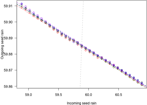
        xlab="Incoming seed rain", ylab="Outgoing seed rain")

abline(0, 1, lty=2, col="grey")

abline(fit, lty=2, col=cols[1])

abline(fit2, lty=2, col=cols[2])

abline(fit3, lty=2, col=cols[3])

abline(fit4, lty=2, col=cols[4])

abline(fit5, lty=2, col=cols[5])

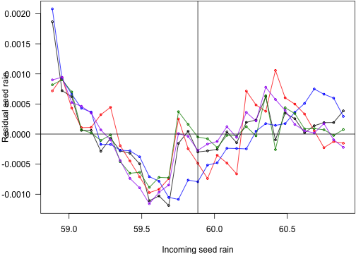
The instability is easier to see here. There are two patterns; the blue and black lines (using the low order integration) have a switch point. The other cases have less systematic error, though general error on the same order. Oddly increasing both the assimilation integration order and the light environment sensitivity did worse than just increasing the light environment sensitivity.

matplot(seed_rain_in,
        cbind(resid(fit), resid(fit2), resid(fit3), resid(fit4), resid(fit5)),
        xlab="Incoming seed rain", ylab="Residual seed rain",
        las=1, pch=1, col=cols, type="o", lty=1, cex=.5)

abline(h=0, v=seed_rain_eq_in)