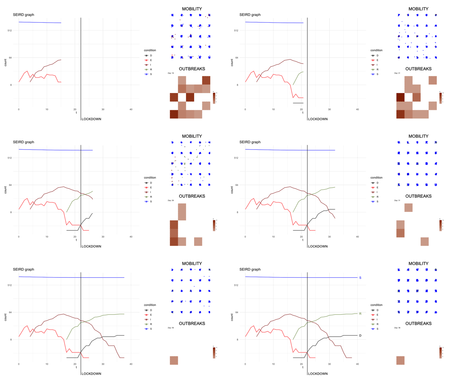
epidsampler is a package for simulate an epidemic map with mobility and social interaction between individuals. Useful for testing sampling methods.
This package was used to perform the simulation in Alleva, Giorgio, et al. "A sample approach to the estimation of the critical parameters of the SARS-CoV-2 epidemics: an operational design" arXiv preprint arXiv:2004.06068 (2020).
This package is in the very early stage of development. It is distributed so users can start to use it and report feedback, but its interface and/or behaviour is likely to change in the future. It is generally best to avoid depending on experimental features.
The package is work in progress and it is not available in the CRAN. However you can install it directly from the github repo.
# The easiest way to get epidsampler is to install it from GitHub:
# install.packages("devtools")
devtools::install_github("vincnardelli/epidsampler")The simulation is divided in two main function. We generate the regular squared lattice grid and the individuals using genmap(). Then, for each day of the simulation (referred as "step"), we simulate the mobility, social interaction and the evolution of the epidemics with the infection and evolution of the disease for each individual in the map.
map <- genmap(n=5, p=c(80, 100))Find out more on the parameter of genmap() in the vignette.
map <- map %>%
    addsteps(n=21, m=0.03, s=2,
             cn=4, cp=2,
             im=3, tE=5, tA=14,
             tI=14, ir=1, cfr=0.15) %>%
    addsteps(n=19, m=0.01, s=1,
             cn=1, cp=2,
             im=3, tE=5, tA=14,
             tI=14, ir=1, cfr=0.15)
Find out more on the parameter of addsteps() in the vignette.
First of all, in order to simulate an artificial population describing the time evolution of an epidemics, we considered a popular model constituted by a system of six differential equations which, in each moment of time, describe six categories of individuals, namely: the susceptibles (S), those exposed to the virus (E), the infected with symptoms (I), those without symptoms (A) and those that are removed from population either because healed (R) or dead (D). The figure below describes diagrammatically the transition between the 6 categories.
Find out more on the parameter of the map generation and the simulation in the vignette.
Vincenzo Nardelli Bicocca University, Milan - vincnardelli@gmail.com
Giorgio Alleva - Sapienza University of Rome
Giuseppe Arbia - Catholic University of the Sacred Heart, Milan
Piero Demetrio Falorsi - Former Director of Methodology at Istat and International Consultant
Alberto Zuliani - Emeritus Professor, Sapienza University of Rome


