README.md

A comparative assessment of machine learning classification algorithms applied to poverty prediction

A project of the World Bank Knowledge for Change (KCP) Program

We provide here a series of notebooks developed as an empirical comparative assessment of machine learning classification algorithms applied to poverty prediction. The objectives of this project are to explore how well machine learning algorithms perform when given the task to identify the poor in a given population, and to provide a resource of machine learning techniques for researchers, data scientists, and statisticians around the world.

We use a selection of categorical variables from household survey data from Indonesia and Malawi to predict the poverty status of households – a binary class with labels “Poor” and “Non-poor”. Various “out-of-the-box” classification algorithms (no regression algorithms) are used: logistic regression, linear discriminant analysis, k-nearest neighbors, decision trees, random forests, naïve Bayes, support vector machine, extreme gradient boosting, multilayer perceptron, and deep learning. More complex solutions including ensembling, deep factorization machines, and automated machine learning are also implemented. Models are compared across six metrics (accuracy, recall, precision, f1, cross entropy, ROC AUC, and Cohen-Kappa). An analysis of misclassified observations is conducted.

The project report is provided in the report folder (ML_Classification_Poverty_Comparative_Assessment_v01.pdf).

As part of the project, a Data Science competition was also organized (on DrivenData platform), challenging data scientists to build poverty prediction models for three countries. Participants in the competition were not informed of the origin of the three (obfuscated) survey datasets used for the competition. One of the three datasets was from the Malawi Integrated Household Survey 2010. We provide in this repo an adapted version of the scripts produced by the 4 winners of the competition (the adaptation was made to make the scripts run on a de-obfuscated version of the dataset).

This project was funded by Grant TF 0A4534 of the World Bank Knowledge for Change Program.

Prerequisites:

The prerequisites for this project are:

• Python 3.6
• pip>=9.0.1 (to check your version, run pip --version; to upgrade run pip install --upgrade pip)

Recommended software:

Although it is not required, we recommend using Anaconda to manage your Python environment for this project. Other configurations, e.g., using virtualenv are not tested. Anaconda is free, open-source software distributed by Continuum Analytics. Download Anaconda for your operating system here. Instructions for environment setup in this README are given for Anaconda.

Setup:

1. Create a worldbank-poverty environment. To do this, after installing Anaconda, run the command:

conda create --name worldbank-poverty python=3.6

After answering yes (y) to the prompt asking you would like to proceed, your environment will be created. To activate the environment, run the following command.

source activate worldbank-poverty

(On Windows, you can just run activate worldbank-poverty instead).

2. Install requirements. First, activate the worldbank-poverty environment and navigate to the project root. If you are using Linux or MacOS, run the command:

pip install -r requirements.txt

If you are using Windows, run the command:

pip install -r requirements-windows.txt

3. Download the data. The data required for these notebooks must be downloaded separately. Currently the Malawi dataset is publicly available through the World Bank Data Catalog. Add raw data to data/raw directory. Extract the contents of all zipped files and leave the extracted directories in the data/raw directory. If you have all the data, then the final data folder will look like:

data/raw
├── IDN_2011
│   ├── IDN2011_Dictionary.xlsx
│   ├── IDN2011_expenditure.dta
│   ├── IDN2011_household.dta
│   └── IDN2011_individual.dta
├── IDN_2012
│   ├── IDN2012_Dictionary.xlsx
│   ├── IDN2012_expenditure.dta
│   ├── IDN2012_household.dta
│   └── IDN2012_individual.dta
├── IDN_2013
│   ├── IDN2013_Dictionary.xlsx
│   ├── IDN2013_expenditure.dta
│   ├── IDN2013_household.dta
│   └── IDN2013_individual.dta
├── IDN_2014
│   ├── IDN2014_Dictionary.xlsx
│   ├── IDN2014_expenditure.dta
│   ├── IDN2014_household.dta
│   └── IDN2014_individual.dta
├── KCP2017_MP
│   ├── KCP_ML_IDN
│   │   ├── IDN_2012_household.dta
│   │   ├── IDN_2012_individual.dta
│   │   ├── IDN_household.txt
│   │   └── IDN_individual.txt
│   └── KCP_ML_MWI
│       ├── MWI_2012_household.dta
│       ├── MWI_2012_individual.dta
│       ├── MWI_household.txt
│       └── MWI_individual.txt
└── competition-winners
    ├── 1st-rgama-ag100.csv
    ├── 2nd-sagol.csv
    ├── 3rd-lastrocky.csv
    ├── bonus-avsolatorio.csv
    ├── just_labels.csv
    └── just_pubidx.csv

The minimum that you need for most notebooks are the 2012 surveys that are contained in data/raw/KCP2017_MP.

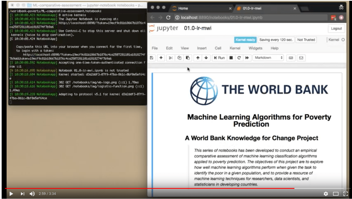
4. Start Jupyter. The Jupyter Notebooks are contained in the notebooks directory. Run jupyter notebook notebooks to access and run the algorithm notebooks that are in the notebooks folder. Jupyter should open a browser window with the notebooks listed. To interact with a notebooks, select and launch (double-click) it from the browser window.

1. Run the data preparation notebooks first. The first notebooks that should be run are 00.0-data-preparation.ipynb and 00.1-new-idn-data-preparation.ipynb. This will read the raw data and output the necessary training and test sets to be used in all of the subsequent notebooks.

2. Run the rest of the notebooks for a first time. After running the data preparation notebook, run the Logistic Regression notebooks first. The notebooks for all other algorithms up to notebooks 12+ compare results to the logistic regression baseline model, so these models must be generated before running other algorithm notebooks. Notebooks 12+ should be run in relative order as well.

3. Explore. After all of the notebooks have bee run once in the proper order, all necessary models and files will have been created and saved, so notebooks can be run in any order. Model files will exist under the models/ directory, and processed data will exist under the data/processed/ directory.

Notes:

• There will be some differences between these notebooks and the published results. Many notebooks have a long runtime when working with the full dataset. The versions that are released include parameters that sample the data or reduce the exploration space. To get equivalent results to the published paper, these notebooks must be executed against the full dataset. Each notebook notes where these parameters can be adjusted to replicate the paper.

---

These materials have been produced by a team at DrivenData.